User Manual — Version 2.401
ProbeItM3 is the Mach3 edition of ProbeIt, a touch-probe program for the Mach3 machine-control software. It runs next to Mach3 and drives it through Mach3’s scripting (COM) interface; nothing is installed into Mach3. It offers some of the same functions as other probing macros:
It also has features that are useful for measuring and reverse engineering:
The goal of ProbeIt is to provide a useful tool with functionality I could not find anywhere else.
ProbeItM3 is a separate program that runs next to Mach3. Start Mach3 first and wait until it has finished loading. Probing uses
Mach3’s own G31 command, in one or two axes at a time, so a probing routine stops by itself when the probe
triggers. You can use other programs while a routine runs: ProbeItM3 does not stop when it loses keyboard focus. Do not jog the machine
or send commands from Mach3 while a routine is running.
/read-only) to look around
and set up without any motion: nothing that moves the machine or changes an offset is then sent to Mach3.I have tried to make the probing routines as safe as I can, but ProbeIt operates your CNC machine through Mach3 and its settings. Setting up Mach3 and the probe input signal is your responsibility. You are responsible for checking and testing all signals and the setup of your machine, and for becoming familiar with the probing routines. When learning, probe items that are not clamped to the table, so that if something goes wrong you are less likely to destroy your probe.
ProbeIt is a tool. It takes your instructions (DRO entries and button clicks), sends commands to Mach3 to move and probe, and saves the data. If you position the probe incorrectly, or issue a G0 that plows the probe through the part, that is on you, and ProbeIt will not prevent it. If you issue a mistaken command, use the Abort button, feed hold, or the E-stop to cancel a running probing event.
Machining is dangerous. Even though ProbeIt is only a probing utility and is not used while cutting, operate the machine as carefully as if you were machining. Never place your hands in the working envelope while probing. Always turn off or disconnect the spindle motor power when a touch probe is mounted. Do not probe at excessive feed rates, and use common sense. By using ProbeIt you accept all liability for damage or harm that could be caused by its use, to you and to your equipment. If you do not agree, do not use this software.
ProbeItM3 is built from ProbeIt for UCCNC, itself a re-write of the original ProbeIt for Mach3, and is still being developed. It is tested to be as free of bugs as possible but it is not guaranteed to work in every setup. CraftyCNC is not liable for any damage or lost time resulting from its use. ProbeIt and CraftyCNC are in no way affiliated with Newfangled Solutions.
ProbeItM3 needs Mach3 3.043.x on Windows 7 or later (32 or 64 bit) with .NET Framework 4.0 or later. It is a separate 32-bit program that attaches to the running Mach3 through its scripting (COM) interface, so there is nothing to install or enable inside Mach3, and it does not matter which profile or screen set you use. Start Mach3 before you start ProbeItM3.
You must have a probe connected and configured in Mach3. The probe does not need to be fancy: it only has to trigger the probe input of Mach3. ProbeIt is best used at a screen resolution of at least 1280 × 1024. Set up the probe input, and check it, before you run any routine: the large Probe Test LED of ProbeItM3 must light when you trigger the probe by hand.
Install with the self-installer ProbeItM3-2.401-Setup.exe. It asks for the folder for the program (default
C:\ProbeItM3). Keep it somewhere you can write to, not Program Files: settings and recorded files are kept below it
(see appendix B). It adds Start Menu shortcuts for ProbeItM3, ProbeItM3 (read-only) and this manual. Your own settings and
recorded files are never replaced by an install or removed by the uninstaller.
To run the installer without prompts: ProbeItM3-2.401-Setup.exe /S /D=C:\ProbeItM3 (/D must be the last argument and
must not be quoted).
The first time ProbeIt runs, and no saved settings are found, it asks whether you work in inch or metric and loads the matching starting values (feed rates, clearances, distances). You can also load an XML file of your own, or skip. All values are only a starting point: please look over every setting and adjust it for your machine, then use Save Settings. You can load either set again at any time with the Set Defaults INCH and Set Defaults MM buttons in the Probe Settings window (see section 8), and save your own as the new defaults (see section 17).
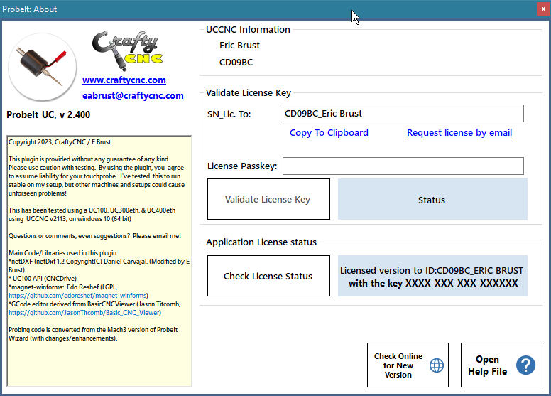
ProbeIt installs in a demonstration mode, so you can try it before buying. The window title bar and the About window show the current status. Demo mode limits only the amount of data that can be recorded; the routines themselves are not crippled:
If you only need the basic probing routines, you do not need a license. If you plan to use ProbeIt for reverse engineering or for business, a license removes every limitation.
To get a license, send an email asking to purchase one, and include the License ID shown in the About window. The passkey is created from that ID, which is made from your Windows installation, your Mach3 license file and the licensee name that Mach3 shows in its title bar. After payment, the passkey is emailed to you. Enter it in the About window and click Validate License Key; the status then shows Licensed.
The Check Online for New Version button in the About window compares your version with the latest one on the CraftyCNC website. The check also runs when the About window is opened, if Auto Check for New Version Enabled is turned on in the General Settings.
Start Mach3 first, load your profile and make sure Mach3 is not in E-stop. Then start ProbeItM3 from the Start Menu. It asks you to confirm that motion is allowed (see section 2.1) and then opens its windows: the main window, the 3D viewer, the status window and, in the main window, the G-code editor. Closing the main window closes them all and stops any jog.
The installer makes two shortcuts: ProbeItM3, which allows motion after the confirmation, and ProbeItM3 (read-only),
which starts the program with /read-only. To use another switch, add it to a shortcut’s target.
| Switch | Meaning |
|---|---|
/read-only | No motion: nothing that moves the machine or changes an offset is sent to Mach3. Positions and state are still shown. |
/maxvel=NNN | Mach3 does not tell programs the maximum speed of its axes. Jog speeds in ProbeItM3 are percentages of this number (default 1000 units per minute): set it to your machine’s real maximum. |
/calibrate | Measure the full jog speed of X, Y and Z by jogging each axis (about 1.5 s, up to 3 in / 76 mm, and back; it asks first). Normally not needed: the speeds are read from the Mach3 profile file (the X, Y, Z velocities in Motor Tuning). /maxvel overrides both. |
/misstol=VALUE | How close to its end point a probe move must finish, with the probe input off, to count as a miss (default 0.002 units). |
/g1jog | Jog with a stream of short G1 moves instead of Mach3’s own jog. It lags; use it only if Mach3’s own jog does not suit your setup. |
/machcoordled=N | The Mach3 LED that shows machine coordinates (default 16). Only needed on an unusual setup. |
/log | Writes every command sent to Mach3 to ProbeItM3.log next to the program (a CSV file), for checking what happened and for support. Off by default. |
/log=PATH | The same, to the file you name. |
/probe[=PATH] | Writes a read-only report of what Mach3 answers (state, positions, probe input, variables) to a text file and exits. Useful when asking for help. |
ProbeIt has three main windows: the main window, the 3D viewer and the status / measurement window. They snap and stick to each other and move as a group when you drag the main window; drag the viewer or the status window away to un-stick them. A pop-up result box shows the measurement of each routine. The settings are in their own windows, opened from the Settings / Help button.
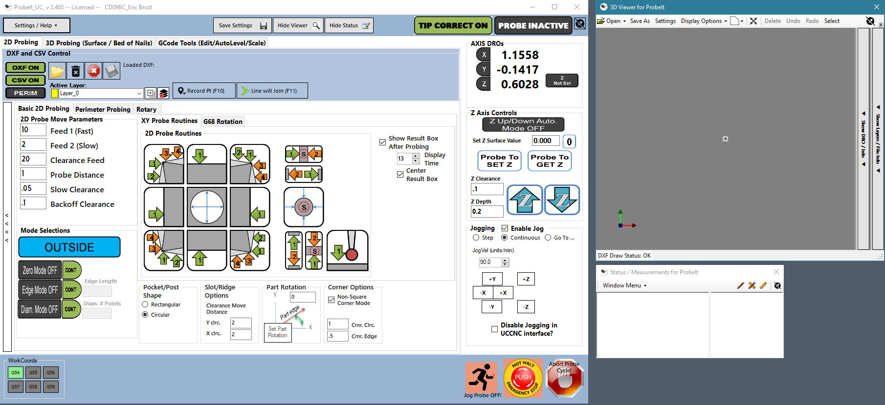
The main window has these tabs,
The probe settings, general settings, email setup and About pages are no longer tabs: they open in their own windows from the Settings / Help button at the top left of the main window (section 6.2).
Always visible, whichever page you are on:
The left panel with the settings of the current page slides open and closed (use the small arrow on its edge); ProbeIt remembers the state between sessions. The probe routine buttons keep a square shape as you resize the window.
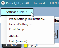
The Settings / Help button opens a menu with:
Each of these windows remembers where you left it, can snap to the other windows, and keeps its settings when you close it with the X (it is just hidden).
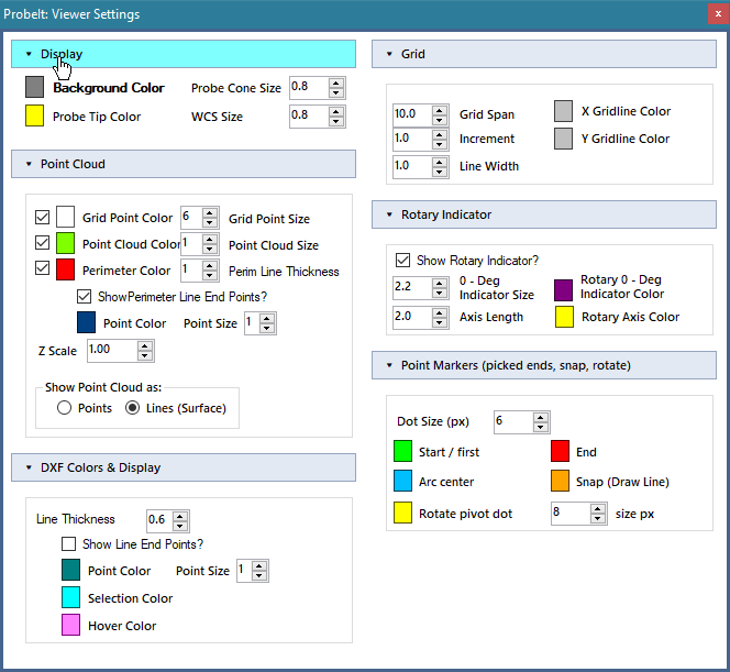
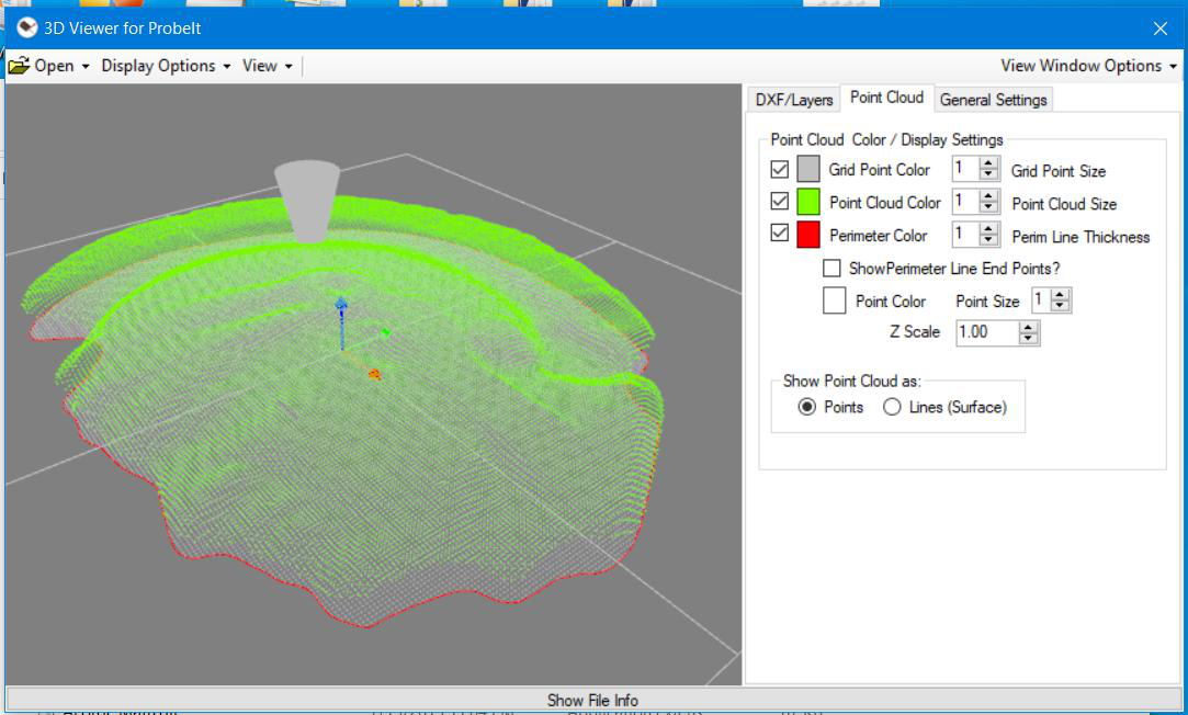
The viewer shows the point-cloud data and the DXF data that you record while probing, and the live probe position. It also
shows information about the DXF file, and has a layer panel to create, rename, delete, hide and color layers and to choose the
active layer that new data is recorded onto (a layer is always selected: ProbeIt picks Layer_0, and makes it if there are no layers). It is the same viewer that UCamCopy uses. You can:
The viewer is not used for G-code; the G-code tab has its own viewer for that.
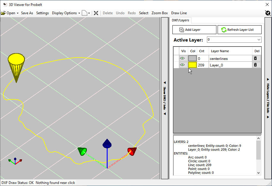
You can clean up the recorded DXF data in the viewer before you save it, and add to it. Everything here works on the DXF data only.
The viewer toolbar holds, from the left:
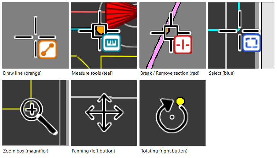
The mouse cursor shows which tool is on. It is a cross-hair, with a small colored badge at its lower right that says what the tool does: orange for Draw line, teal for the eight Measure tools, red for the cutting tools (Break at point, Remove section) and blue for Select. Zoom box shows a magnifier. When the pointer is on something a click will use (a snap point, or a circle, arc or line for the tools that click a shape) a small square appears around the middle of the cross-hair. While you pan (left button) the cursor becomes four arrows, and while you rotate (right button) it becomes a circular arrow; the tool’s cursor comes back when you let go. With no tool on, the cursor is the normal arrow.
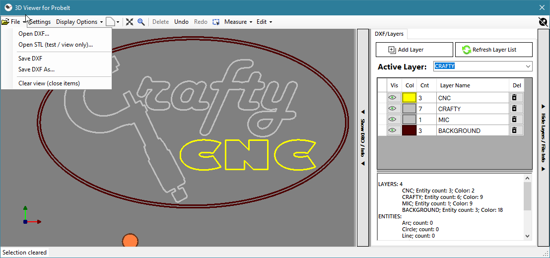
Click a line, circle, arc or polyline to select it; it is drawn in the Selection Color (cyan by default). Ctrl-click or Shift-click adds an entity to the selection, or removes it if it is already selected. To select many at once, click the Select button on the toolbar (the dashed box) and drag a box: everything the box touches is selected (hold Ctrl or Shift to add to the selection, Alt to remove from it). The Zoom box button (the magnifier, next to Fit) works the same way but zooms to the box. Esc clears the selection.
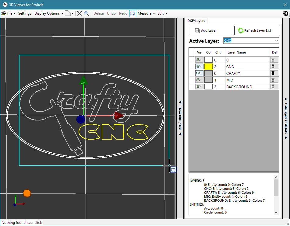
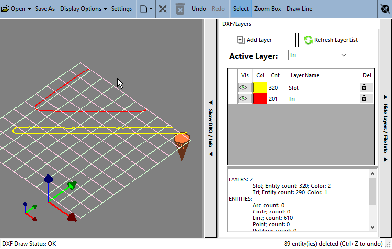
With entities selected, click Delete (or press Delete) to remove them from the DXF data. Undo (Ctrl+Z) takes back the last change and Redo (Ctrl+Y) puts back what you undid; the history covers deleting entities, drawing lines and moving entities to another layer. Any edit marks the DXF as having unsaved changes, so the Save button on the main window becomes available.
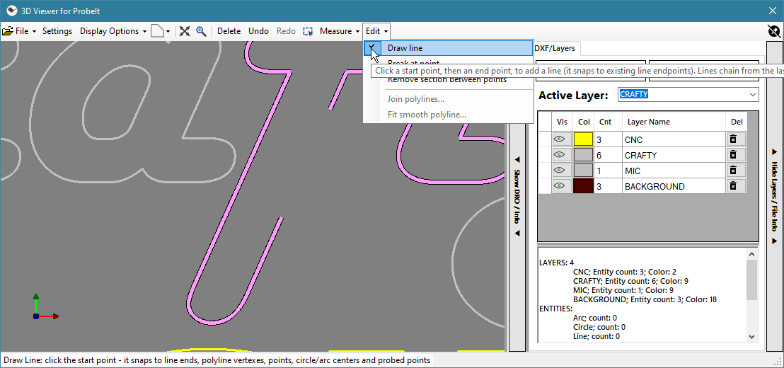
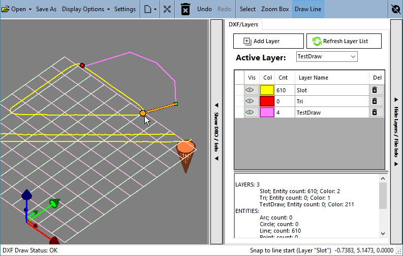
Draw Line adds new lines to the DXF by clicking in the view. Choose Draw line in the Edit menu on the toolbar (it stays checked while the tool is on), click the start point (a green dot marks it), then click the end point. A line is added, and its end point becomes the start of the next line, so you can keep clicking to draw a connected series. A thin orange rubber-band line follows the pointer from the start point: it is dashed while the pointer is on a free spot, and solid once the pointer is on a snap point, so you can tell at a glance whether the click will snap. Press Esc once to end the series and again to leave the tool; choosing it again also turns it off. Use the Top view for drawing: in an edge-on view such as Front or Right a click cannot be placed on the Z = 0 plane.
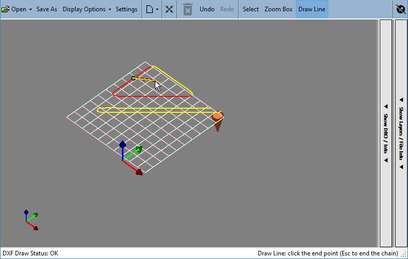
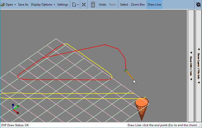
Snapping: within about 12 pixels of a snap point, an orange dot appears on it and the status bar names it. The point you click is then exactly that point, so lines join cleanly. The snap points are the same as for Measure (below): the ends of lines, DXF points, the centers of circles and arcs, the ends of arcs, the vertexes of polylines, and probed perimeter, grid and point-cloud points. Away from a snap point the point is where you click, at Z = 0.
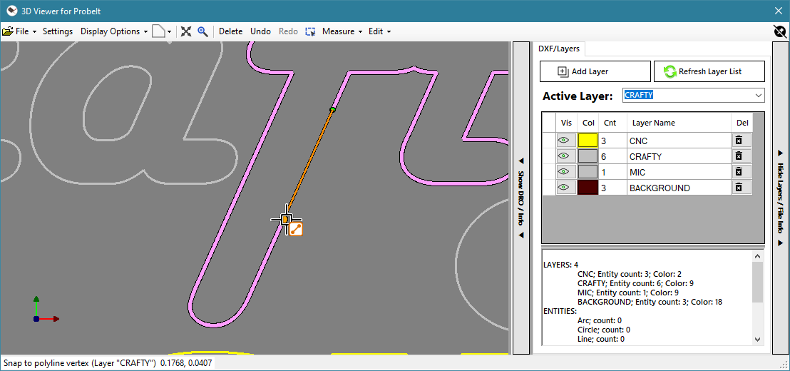
New lines go on the active layer. Each line is one Undo step.
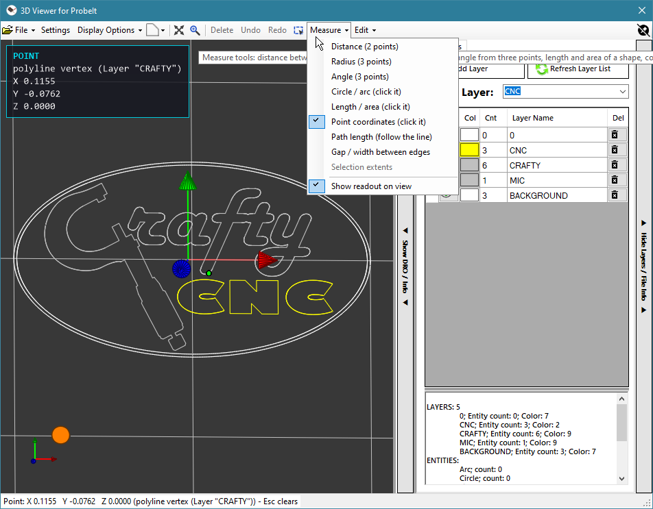
The Measure button on the viewer toolbar is a menu of measuring tools; it is also in the right-click menu as Measure. Choose a tool from it. The tool stays on until you press Esc twice or choose it again, and while it is on you can still pan, rotate and zoom the view. The tools measure in the X/Y plane and ignore Z, so use the Top view. There are eight tools and one command:
Only geometry counts. The five tools that take points (Distance, Radius, Angle, Point coordinates and Path length) only accept snap points; a click on empty space does nothing. An orange dot shows the snap point under the pointer, and the status line below the view names it. The snap points are the ends of lines, DXF points, the centers of circles and arcs, the ends of arcs, the vertexes of polylines, and the points of a probed perimeter, grid, rotary grid or point cloud (the data you see in the viewer, whether or not it has been saved to a DXF). Only layers that are shown can be snapped to. The snap target is the nearest one within about 12 pixels of the pointer.
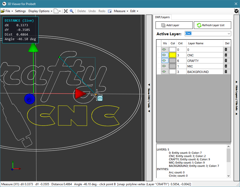
Distance (2 points). Click point A (a green dot) and then point B (a red dot). After A, a thin teal line follows the pointer (dashed on a free spot, solid on a snap point) with dotted lines showing the dX and dY parts; the click still only counts on a snap point. A line joins A and B once both are set, and the result is the difference in X (dX), the difference in Y (dY), the straight-line Distance between the two points in the X/Y plane, and the Angle of the line from A to B in degrees. While you move toward B, the status line shows the same numbers for the point under the pointer. If the two points are at different heights (for example probed grid points) the readout panel also shows dZ and labels the two distances: Dist2D is the distance in the X/Y plane (the one the status line and the measurement window report, with the Angle), and Dist3D is the straight-line distance that includes the height difference. A third click starts a new measurement at a new point A.
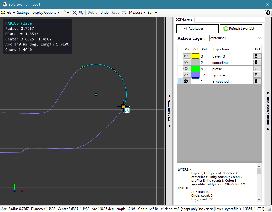
Radius (3 points). Click three snap points that lie on an arc or a circle. The circle through them is worked out and drawn on the arc from the first point, through the second, to the third, with a blue dot on its center. After the first point a dashed guide line follows the pointer. After two points, the circle through them and the pointer is previewed as you move (dashed on a free spot, solid on a snap point), and the status line shows its radius; the third click must be on a snap point. The result is the Radius, the Diameter, the Center (X, Y), the Arc angle and length (measured along the arc from the first point to the third, passing through the second) and the Chord (the straight distance from the first point to the third). If the three points are in a line there is no circle, and the viewer asks for a different third point. A fourth click starts a new measurement. The radius is that of the points you picked; to measure a probed circle or arc, pick points on it that were probed.
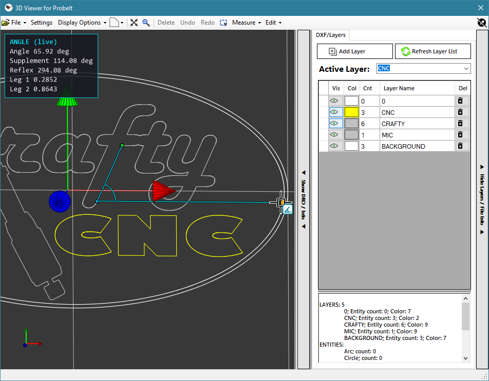
Angle (3 points). Click three snap points in this order: the start point (a green dot), the vertex, which is the corner of the angle (a blue dot), and the end point (a red dot). The two legs are drawn from the vertex, with a small arc between them. After the vertex, moving the pointer previews the angle live, free or on a snap point. The result is the Angle between the two legs (0 to 180 degrees), its Supplement (180 minus the angle), the Reflex angle (360 minus the angle) and the lengths of Leg 1 (vertex to start point) and Leg 2 (vertex to end point). The angle is the one between the legs, so it never depends on the order you picked the start and end points. A fourth click starts a new measurement; Esc clears the points and Esc again leaves the tool.
Circle / arc (click it). Move the pointer onto a circle, an arc or an arc segment of a polyline (a rounded corner or curve in a polyline, such as the ones Fit Polyline makes). It is highlighted, and the status line already shows its measurements. Click it to keep them: the highlighted shape stays in the selection color with a blue dot on its center, and the line is written to the measurement window. For a circle the result is the Diameter, Radius, Center and Circumference; for an arc it is the Radius, Diameter, Center, the Arc angle (with the angles it runs from and to, counter-clockwise from the X axis) and length, and the Chord. This measures the stored geometry, so it needs no snap points. A click on empty space does nothing, and only layers that are shown can be picked.
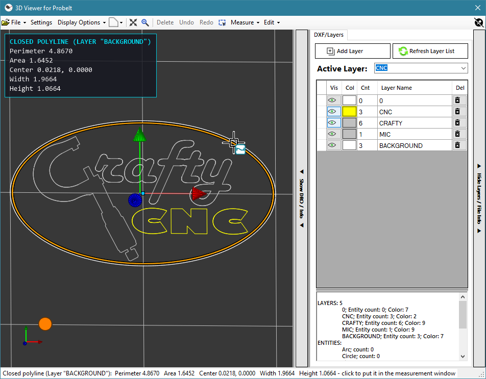
Length / area (click it). Move the pointer onto a line, arc, polyline or circle: the whole shape is highlighted and the status line and the readout panel show its numbers; click it to keep them (the shape stays highlighted, and a closed shape gets a blue dot on its center). For a line, an arc or an open polyline the result is its Length (along the arcs too), the Chord (the straight distance from its start to its end) and its Width and Height (the size of the box that holds it). For a closed polyline it is the Perimeter, the Area, the Center of the area and the Width and Height; for a circle it is the Circumference, Area, Diameter and Center. Arcs inside a polyline are counted exactly. To measure an outline that was recorded as many short lines, first join it into one polyline with Join polylines (or Fit smooth polyline). Lengths and areas are in the X/Y plane. This works on the stored geometry, so it needs no snap points.
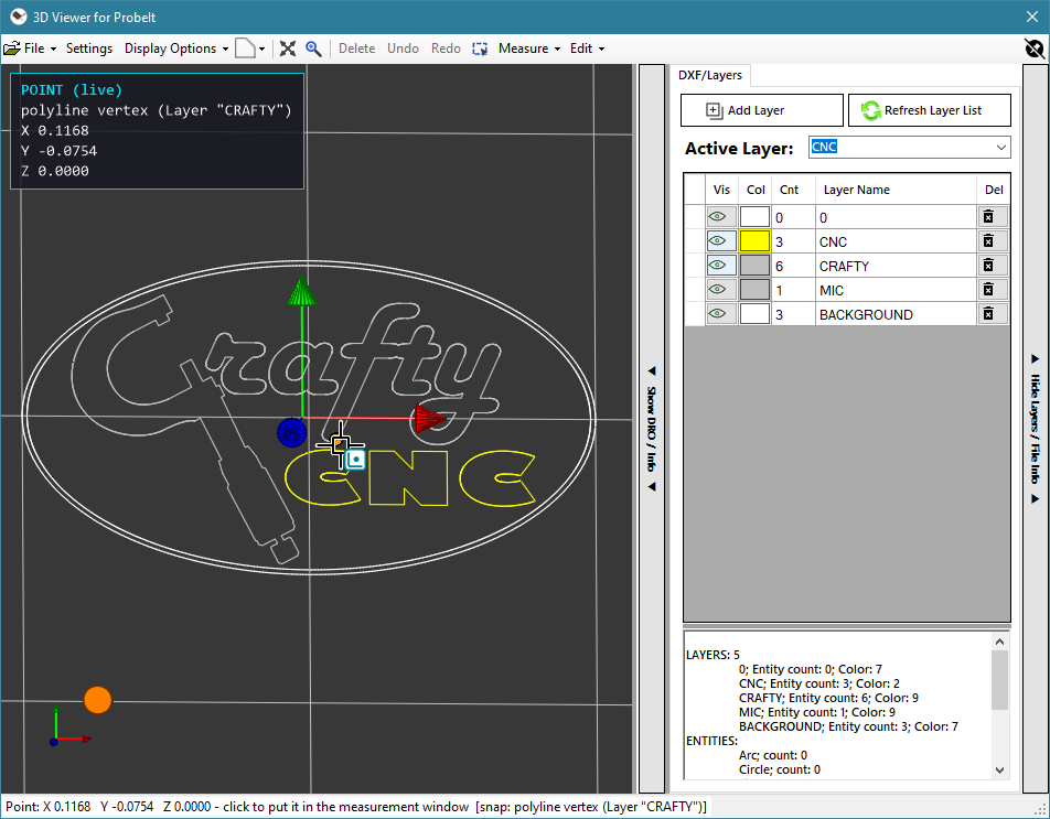
Point coordinates (click it). Move onto a snap point: the status line and the readout panel show its X, Y and Z and what it is (a line end, a circle center, a probed point, and so on). Click it to keep it: a green dot marks the point and the coordinates are written to the measurement window. A click on empty space does nothing; Esc clears the point and Esc again leaves the tool.
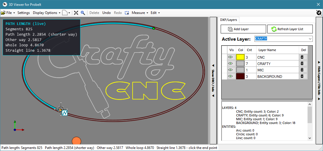
Path length (follow the line). For an outline recorded as many small segments. Click a start point on the outline (a green dot; any line end, arc end or polyline vertex of it), then an end point further along it. ProbeIt joins up the connected lines, arcs and open polylines (pieces whose ends meet within a small gap, 0.01 by default) and measures the length of the segments between the two points, following the shape, not the straight line between the clicks. After the start point, moving the pointer onto another snap point on the same outline highlights the path in teal and shows its numbers live in the readout panel: the number of Segments, the Path length (arcs counted exactly) and the Straight line distance between the two points. Click the end point to keep the result (a red dot marks it); it is written to the measurement window. On a closed outline there are two ways round: the shorter one is highlighted and measured, and the panel also shows the Other way and the Whole loop. If the end point is not on the same connected outline (the line has a gap bigger than the join gap), the panel says it is not connected. Lengths are in the X/Y plane. Esc clears the path and Esc again leaves the tool.
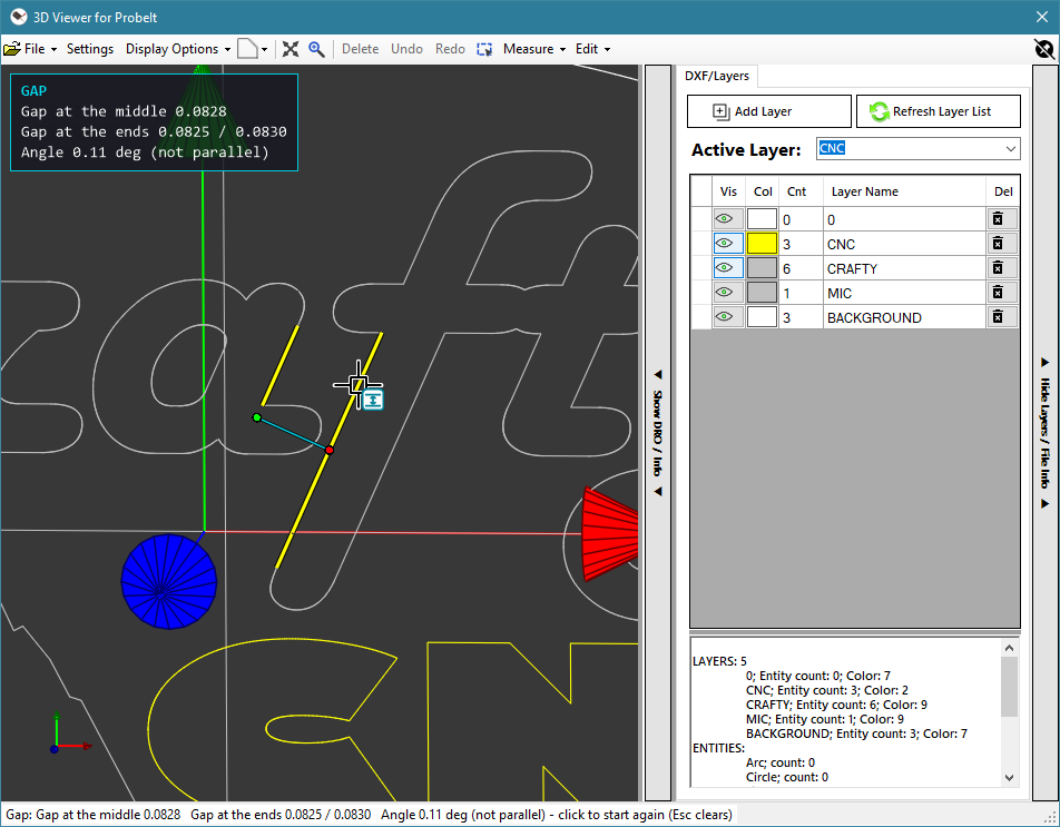
Gap / width between edges. Move the pointer onto a line, or onto a straight segment of a polyline (arc segments are skipped): that edge is highlighted. Click it as the first edge, then move onto the second edge. The panel shows the gap live, and a dimension line is drawn across it with a green dot where it meets the first edge and a red dot at the middle of the second. Click the second edge to keep the result; it is written to the measurement window. The Gap is the perpendicular distance from the middle of the second edge to the (extended) line through the first, so it is the true width when the two edges are parallel. If they are not parallel by more than a twentieth of a degree, the panel instead shows the Gap at the middle, the Gap at the ends of the second edge and the Angle between the edges, so a slot that is wider at one end shows. Lengths are in the X/Y plane. A click on empty space does nothing; a third click starts again, Esc clears the edges and Esc again leaves the tool.
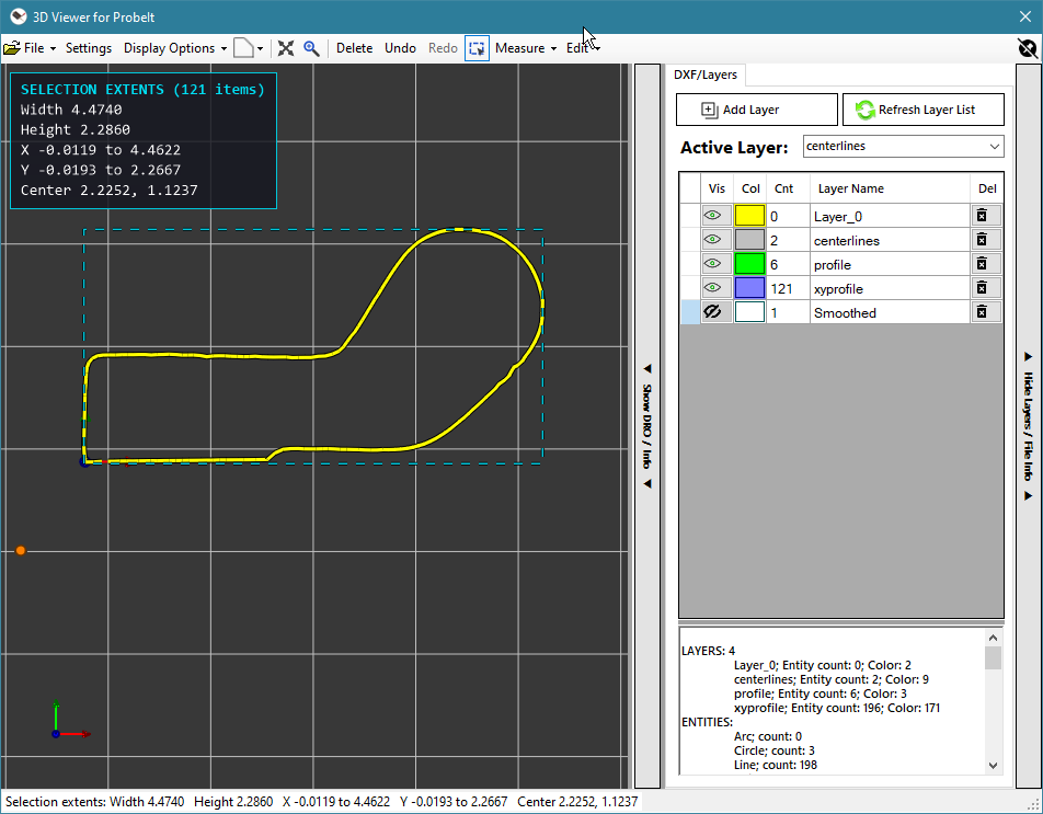
Selection extents. Select one or more items (click them, or use the Select tool and drag a box), then choose Measure > Selection extents (it is greyed out until something is selected; it is also in the right-click menu). A dashed box is drawn round the selection and the readout panel shows the Width and Height of the box, its X and Y ranges, its Center and, if the items are at different heights, the Z range; the numbers are also written to the measurement window. Lines, arcs, circles, polylines and points count (arcs and circles by their whole outline). The box and the numbers stay until you change the selection. Because it works on the selection, it needs no clicking on snap points, and it works with any tool or none.
The readout panel. While a measurement is in progress a small dark panel in the top-left corner of the view shows its numbers, updated as you move the pointer: dX, dY, Dist and Angle for a distance (it keeps showing the finished measurement until you clear it with Esc or leave the tool), the radius, diameter, center, arc angle and length for a 3-point radius, the angle, supplement, reflex and leg lengths for an angle, the diameter, radius and center of the circle or arc under the pointer for Circle / arc, the length or perimeter and area of the shape under the pointer for Length / area, the coordinates of the snap point for Point coordinates, the length along a connected outline for Path length, the gap and angle between two edges for Gap / width, and the size of the box for Selection extents. The title says (live) while the numbers are following the pointer. Choose Show readout on view at the bottom of the Measure menu (toolbar or right-click) to switch the panel off or on; the choice is remembered. The numbers are also written to the status line and to the measurement window.
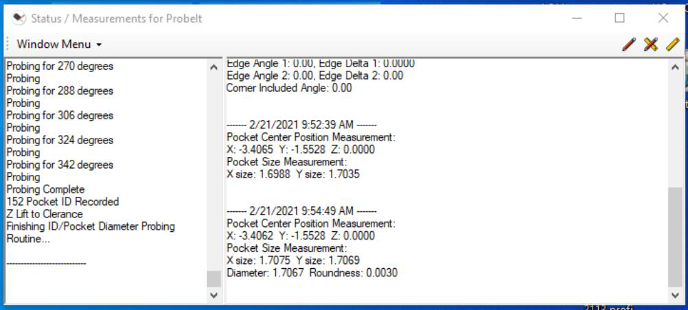
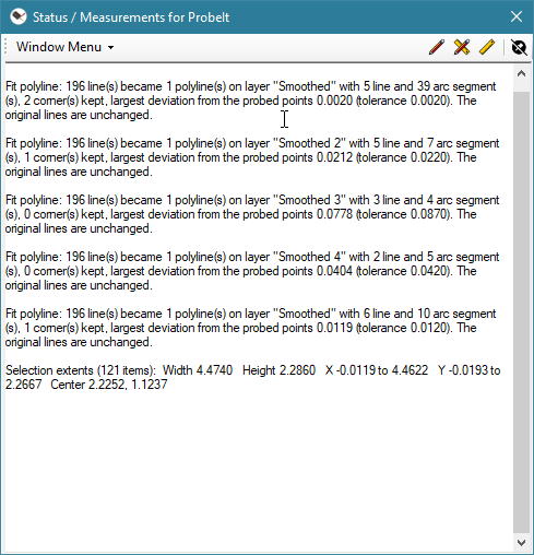
Where the results go. Each finished measurement is written to the measurement half of the status / measurement window (section 6.4), the same place the probe measurements go, with a blank line before it so the results are easy to tell apart. They can be copied, e-mailed or saved from that window like the probe results. If the General Settings send status messages to Mach3’s own status box instead, the result goes there. The status line of the viewer also shows the result until you move on. Esc clears the measurement in progress; pressing it again leaves the tool.
A perimeter is recorded as many short straight lines, one for every probed point. Fit Polyline cleans that up: it replaces the outline with a short polyline of straight segments and arcs that follows the probed points, with the sharp corners kept sharp. Use it to get a clean outline for a CAD or CAM program, or to read off radii with the Circle / arc measure tool.
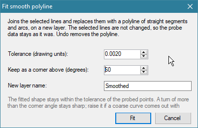
The selected lines are not changed, so the probe data is still there, on its own layer; hide that layer to see only the clean outline. The new polyline is selected, and a line in the measurement window says how many lines became how many polylines, how many straight and arc segments there are, how many corners were kept, and the largest distance between the probed points and the new shape (it is never more than the tolerance). Undo (Ctrl+Z) removes the polyline.
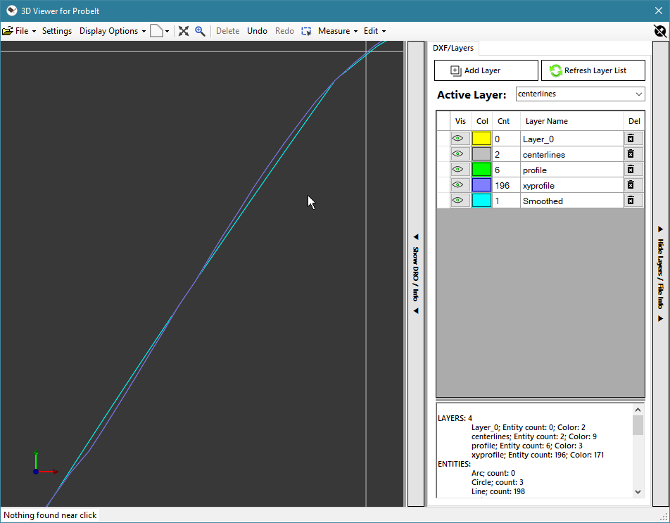
Lines that join end to end are fitted as one polyline each, whatever order or direction they were drawn in, so several separate outlines selected together give several polylines. A loop that comes back to its start becomes a closed polyline. One arc segment is at most a half circle, so a full circle becomes two arcs. The viewer draws polylines flat at Z = 0, and the polyline stores the average height of the lines it replaces.
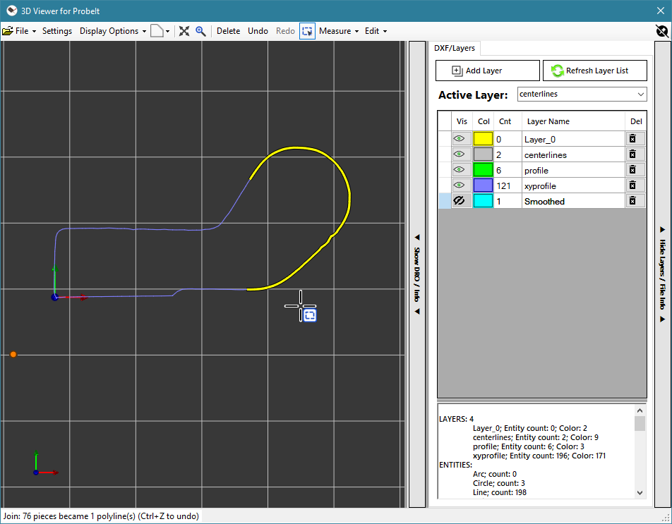
Join turns pieces that meet end to end into one polyline: for example the lines and polylines of an outline that was probed in several runs, or drawn in several pieces.
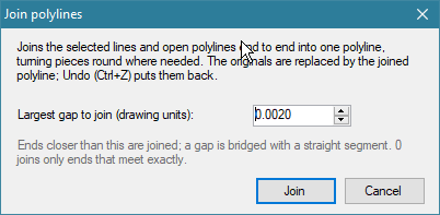
Pieces drawn in different directions are turned round as needed (the arcs in a polyline keep their shape). A joined path that comes back to its start becomes a closed polyline. The joined polyline replaces the pieces and goes on the layer of the first piece; pieces with nothing within the gap are left alone, and closed polylines cannot be joined. The status line says how many pieces became how many polylines, and Undo (Ctrl+Z) puts the original pieces back.
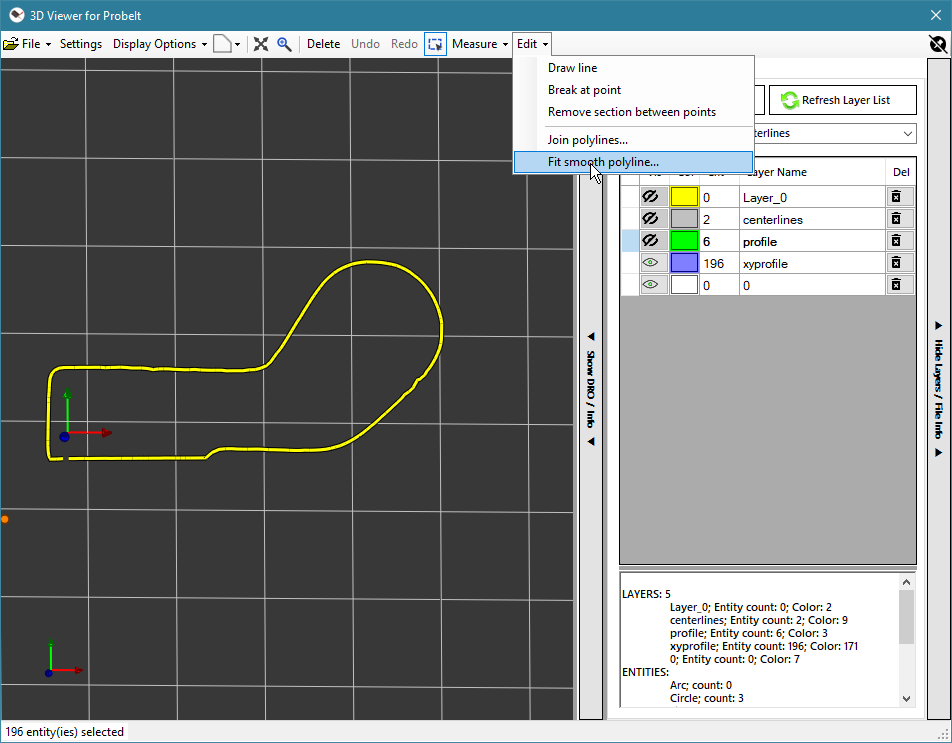
The Edit menu on the viewer toolbar (and Edit in the right-click menu) holds the tools that change the drawing: Draw line (above), Break at point and Remove section between points (below), and Join polylines… and Fit smooth polyline… (which work on the selected lines and polylines, and are greyed out until some are selected). The two cutting tools work on the shape under the pointer, so nothing needs to be selected first, and they work on the lines, arcs and polylines of any layer that is shown (a circle is not cut). A cut replaces the shape with its pieces on the same layer, and Undo (Ctrl+Z) puts the original back. A click on empty space does nothing.
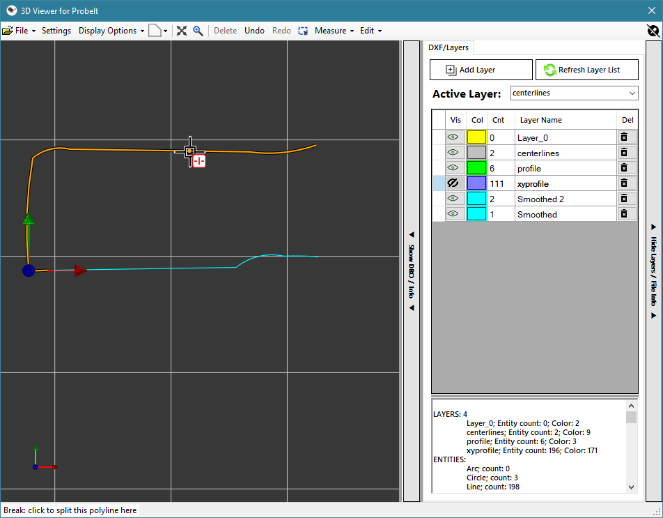
Break at point. Move the pointer onto a line, arc or polyline: it is highlighted, and an orange dot shows the spot, which is anywhere along the shape. When the pointer is near one of its vertexes (the corners and ends of a polyline) the dot jumps to that vertex and gets larger. Click to split the shape there:
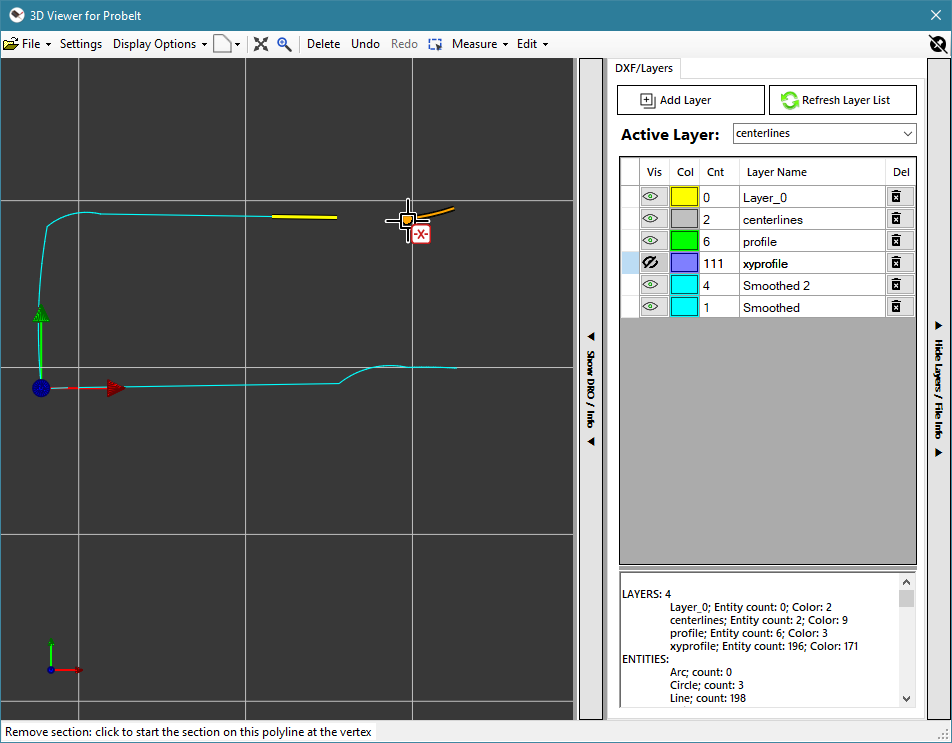
Remove section between points. Click where the section starts (a green dot marks it) and then, moving along the same shape, where it ends. Before the second click the part that will be removed is highlighted in red, and the status line says what a click will do. Clicking removes it and leaves the rest:
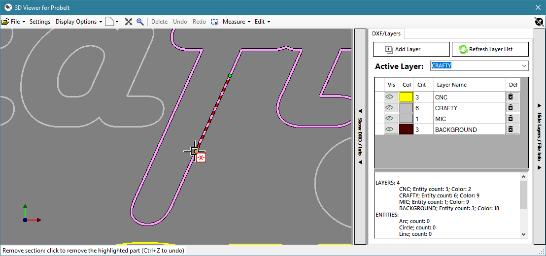
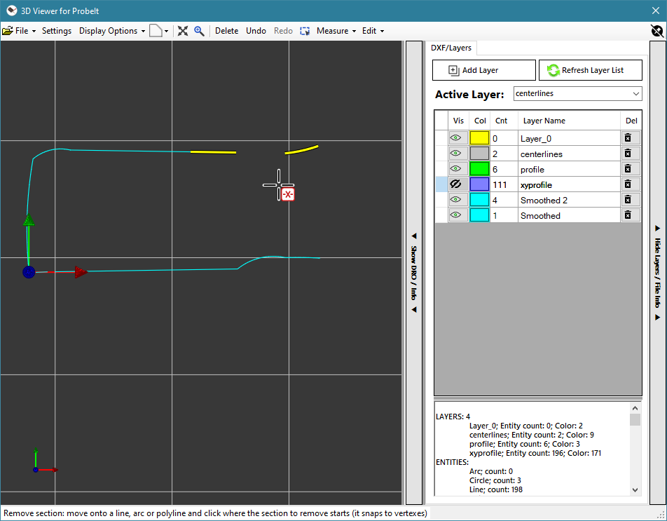
The two points can be clicked in either order. A line stays a line, an arc stays an arc and a polyline stays a polyline. Press Esc to drop the first point, and again to leave the tool.
The layer list has these columns: Vis (click to show or hide the layer), Col (double-click to change its color), Cnt (the number of entities on it), Layer Name (edit it to rename the layer) and Del (delete the layer and its entities, after a confirmation). A layer whose color is 7 (white, or black on a light background, in most CAD programs) is drawn black when the viewer’s background is light, so its lines stay visible. Add Layer (or New Layer… in the right-click menu) asks for a name and then a color; Refresh Layer List rebuilds the list. Layer names must be unique (upper and lower case count as the same): a name that is already in use is refused, both for a new layer and when renaming.
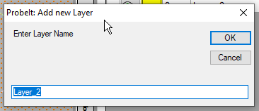
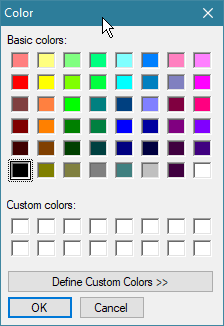
To move entities to another layer, select them, right-click one of them, choose Move to layer and pick the destination layer. The entities keep their positions; only their layer changes, and Undo moves them back.
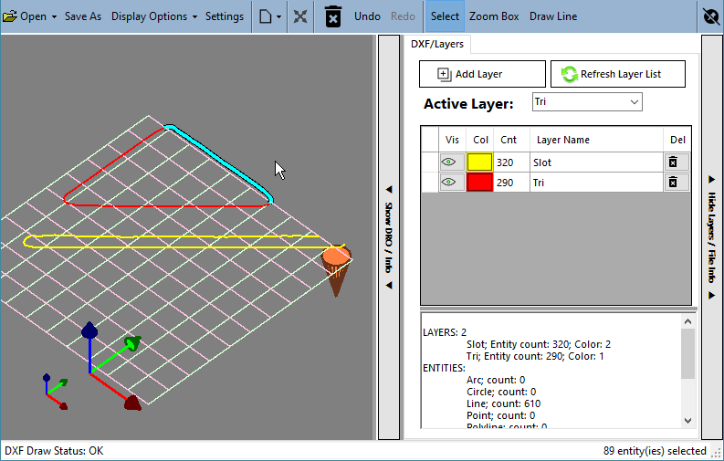
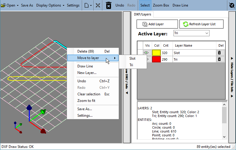
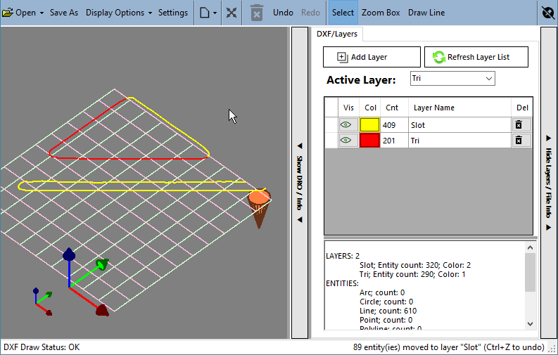
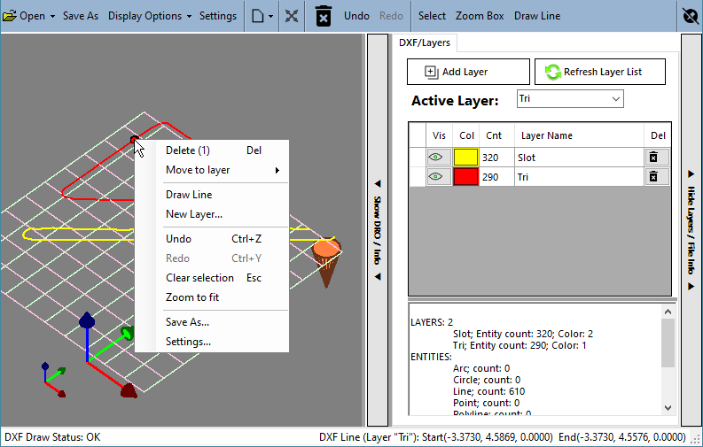
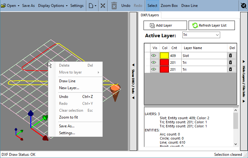
Right-click (without dragging) in the 3D view to open a menu. If you right-click an entity that is not selected, it becomes the selection; if it is already part of the selection the whole selection is kept, so you can act on a group. The menu has Delete (n), Move to layer, Measure (with Distance, Radius, Angle, Circle / arc, Length / area, Point coordinates, Path length, Gap / width, Selection extents and Show readout on view), Edit (with Draw line, Break at point, Remove section, Join polylines… and Fit smooth polyline…), New Layer…, Undo and Redo, Clear selection, Zoom to fit, Zoom box, Save As… and Viewer Settings…. Entries that do not apply, such as Delete with nothing selected, are greyed out.
The status window collects status information while you probe (left half) and builds a measurement report for the 2D routines (right half), which also collects the results of the viewer’s Measure tools (section 6.3). Buttons show only the status, only the measurements, or both. You can copy both, e-mail them or save them to a text file, and type your own notes next to the results. The Status Messages option in the General Settings chooses whether status messages go to this window or to Mach3’s own status line.
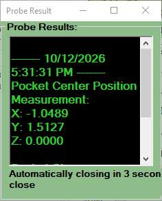
After a routine, a pop-up result box shows the measurements. It can use your choice of font and background colors (set in the General Settings), stays open for a time you set, opens at the size and place where you left it, and stops auto-closing if you click it. The Show Result Box check box and the display time are on the XY Probe Routines page.
The Abort button stops the running probe routine. It is gray when no routine is running and yellow while a routine is running and the button can cancel the motion. You can also use feed hold or the E-stop; after a reset, you can always restart the probing. If the button does not turn gray after you click it, the program may be hung and need a restart.
Feed rates and distances are typed in the units that Mach3 is set up for (inch or mm; feed rates per minute). There is no unit conversion in ProbeIt: a value of 1 is one inch if Mach3 is in inches and one millimeter if Mach3 is in metric. This is also true of the recorded files (section 13).
Positioning before probing is done manually, by jogging. Placing the tip is not critical: make sure it is closer to the part than the max probe distance. If you use the auto Z up/down feature the tip can be left above the surface; after the Z surface is touched off and set, the probe moves down automatically before, and up after, each probe event. You can use a pendant, an Xbox controller or the jog buttons in the program.
When you open a file to record to, you can start and stop recording as needed. You can probe a perimeter, jump to the XY page and record a bore, set a new Z, return to the perimeter page and record another perimeter, all into the same file. When you are done, close and save the DXF file. If you were also recording a CSV and a perimeter file, they are saved with the same name.
The Probe Settings window (Settings / Help → Probe Settings (calibration)…) is mainly for calibrating the probe tip, which builds a table of corrected tip diameters at various probing angles. Using the table corrects for:
The probe’s contribution may not be the same in all directions, so install your touch probe in the same orientation every time (for example, so that the lead always exits in the same direction).
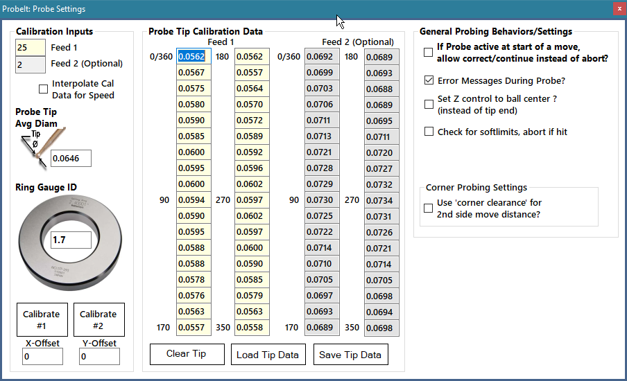
Calibrate the probe
You calibrate with a master ring gauge of known inner diameter. Calibration is optional: you do not have to calibrate to run any of the probing routines, but you must enter a value in Probe Tip Avg Diam, which is used as the default tip diameter.
Save Tip Data saves the tables to a file you name, useful if you alternate between several tips or probes; Load Tip Data asks for the name of a saved file (you have to type the name) and fills in the tables and the Avg Diam box. Clear Tip Data empties the tables.
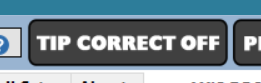
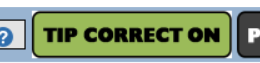
Click the Tip Correct button to turn tip correction on or off. Leave it on once you have calibrated and the table is correct, and off if the table is out of date (for example you just changed the tip and did not recalibrate). With correction off, the Avg Diam value is used for every probe event. Starting a calibration turns it off until the routine completes.
The Set Defaults INCH and Set Defaults MM buttons reload the starting values for the units you choose (they also reset the viewer’s grid and marker sizes to match), and Open Settings XML File loads a settings file you choose. Use Save Settings afterwards to keep the values.
These settings appear on several pages. Feed rates are in your native units per minute, distances in your native units:
| Input | Meaning |
|---|---|
| Feed 1 (initial feed) | The feed rate at which the probe travels during a probe operation. Start slow and increase to your comfort and accuracy level. |
| Feed 2 (slow feed) | A second, slower feed: the probe travels at Feed 1, backs off, then re-probes at Feed 2. Set to 0 for no second slow probe. Recommended: 1–5 in/min (25–125 mm/min). |
| Clear feed | The feed for clearance moves, such as moving along an edge between points or around a corner. |
| Slow clear | How far the probe backs off before the slow probe. Ignored if Feed 2 is 0. |
| Probe distance (max distance) | How far the probe will travel toward the surface. With the hit tolerance, it decides whether the surface was hit or missed. |
| Backoff clearance | How far the probe backs away from the touched surface before a clearance move. |
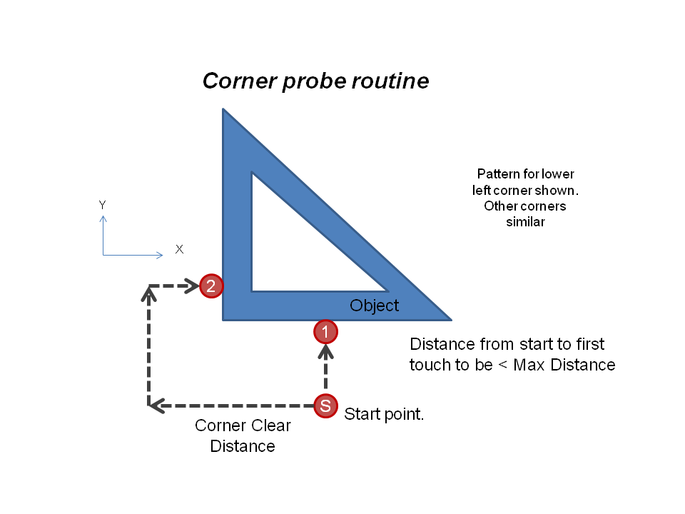
| Corner clearance | How far the probe travels to get around a corner. Make it larger than the distance from where you start probing to the corner. |
The XY Probe Routines page can serve several purposes. For general probing and setup work it locates edges, corners, bore or post centers and slot mid-points, and sets the coordinates. It reports measurements: point location (edge and corner), diameter and roundness (bore and post), width or height (pocket, slot, ridge) and angle (edge). For reverse engineering it complements the perimeter routine: with DXF or CSV recording on, the routines record their data, and you can jump between the perimeter page and the XY page and record all the geometry in one file.
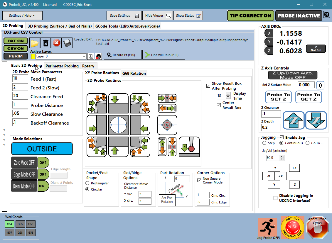
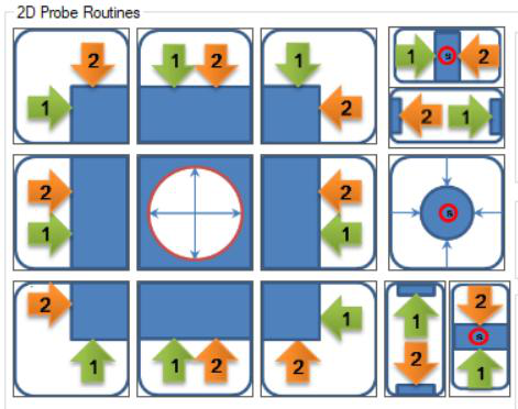
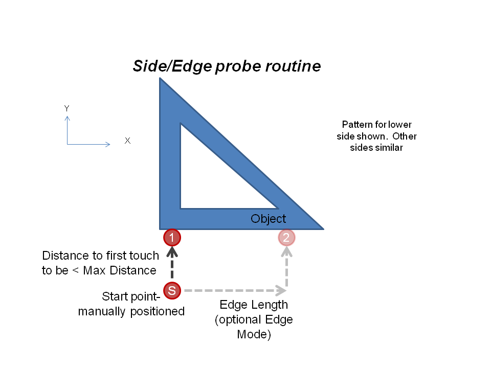
These buttons probe a side, or an edge if edge mode is on. Edge mode measures the slope of the side (two points); probing a side returns the X or Y point touched. If zero mode is on and edge mode is off, the X or Y axis is zeroed (depending on whether you probe horizontally or vertically). The part rotation value modifies the event, and auto up/down can be on.
During an edge move, if the Edge Length is positive the probe moves from 1 to 2 as pictured on the button; if it is entered negative, the order is reversed, from 2 to 1.
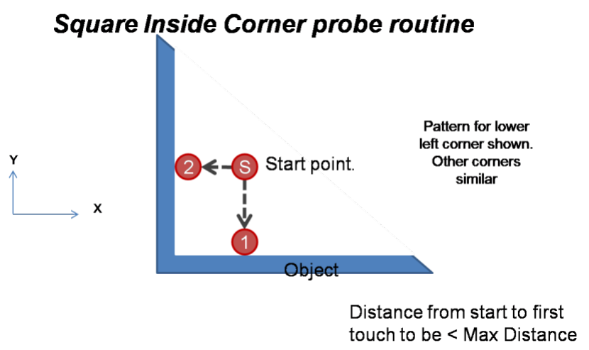
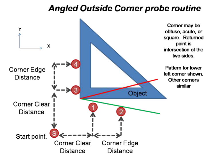
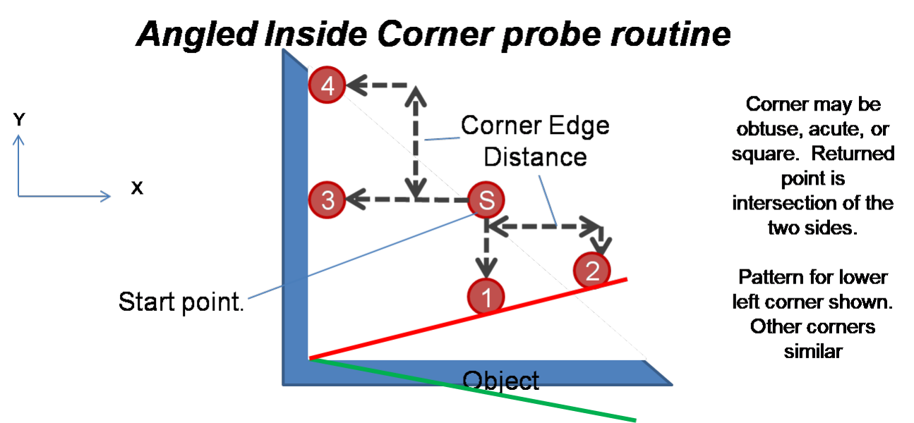
Choose inside or outside, and square or angled corners, with the Corner Options (Non-Square Corner Mode, Inner / Outer, Cmr. Clrc. and Cmr. Edge). The returned point is the intersection of the two sides, the exact corner, and can be set to X0 Y0 if zero mode is on. Corner routines are modified by part rotation and can use auto up/down. Position the probe closer to the corner than the corner clearance value.
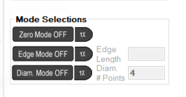
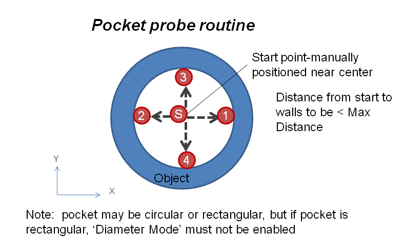
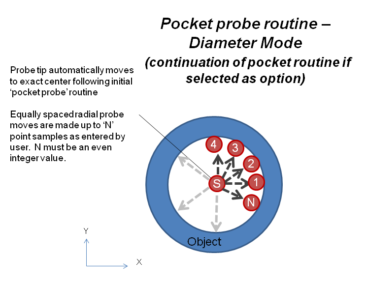
The probe bore button probes the inside of a round bore or a rectangular pocket. Put the tip near the approximate center in XY. With Diameter Mode in Holes off, the routine finds the center of a bore or rectangular pocket, probing ±X and ±Y only; if DXF recording is on, a circle or a rectangle is recorded depending on the Pocket / Post Shape option (rectangular or circular). With diameter mode on, it finds the center of a round bore and then samples the ID at as many points as you enter in Diam # Points, returning a measured diameter and roundness and recording a circle.
This event is modified by part rotation (if diameter mode is off) and can use auto up/down.
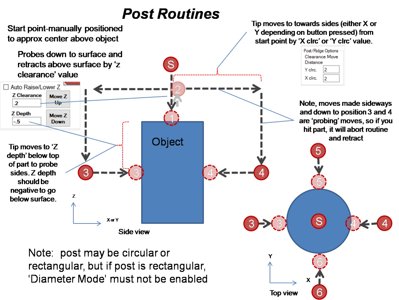
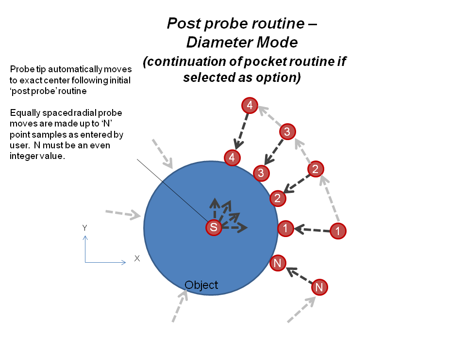
The probe boss button probes the outside of a post. Put the tip above the approximate center of the post, a small amount above it. With diameter mode off, the routine finds the center of a boss or rectangular post, probing ±X and ±Y; if DXF or CSV recording is on, you are asked whether the post is round or rectangular, so that the right geometry is recorded. With diameter mode on, it finds the center, then samples the OD at Diam # Points points.
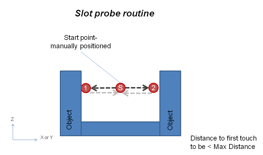
Slot. Start with the probe approximately centered in the slot. The probe makes moves to probe both sides, then returns to the exact center of the slot, and returns the width or height and the center position. Modified by part rotation; can use auto up/down.
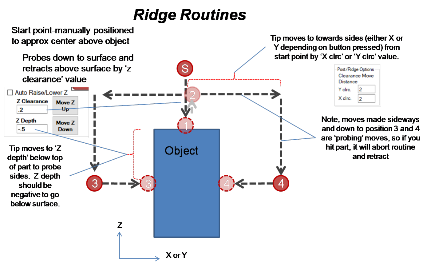
Ridge. Start with the probe approximately centered above the tab or ridge. The probe first goes down to find the top of the ridge, then makes moves to probe both sides, and returns to the exact center above the top surface; width or height and center position are returned. Modified by part rotation. A ridge routine cannot run with auto up/down: if it is on when you start, it is turned off. Use Y clrc. and X clrc. (Post / Ridge options) to set how far the tip moves to the sides.
Probes a Z surface and gets its height without changing the Z Is Set LED or the Z Surface Value. If zero mode is on, it also zeros the Z axis DRO (and if Z Is Set was on, it is cleared by the zeroing).
Each mode button has a Cont. check box: when it is checked, the mode stays on; when it is not, the mode turns off after one routine.
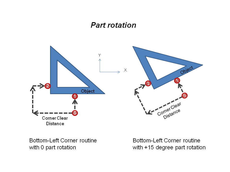
The part rotation value modifies the orientation of all probing events except edge and diameter modes. Use it when your part is not square to the table, or when you have rectangular pockets or corners that are not square to the table. Enter the angle in degrees, positive for counter-clockwise. +X is 0 degrees, and the angle is that of the part’s bottom edge relative to the X axis. Part rotation also rotates the features that are recorded to DXF.
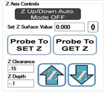
Initial Z surface (Probe To SET Z). Sets the Z axis DRO to a value that represents the surface of your object (its top, for example). The value is what you enter in Set Z Surface Value. Move the probe above the surface first. The button works with the Z Is Set LED: if the LED is on, pressing the button turns it off and you must touch the surface again; if it is off, the routine probes down until it touches, sets the Z DRO to the Z Surface Value, and retracts to the Z Clearance. Example: to make the Z DRO 0 on a surface, enter 0 in Set Z Surface Value and press Probe To SET Z.
Probe To GET Z. Probes down to a new surface (a flange, another level) and puts the measured Z into the Z Surface Value box. It requires that an initial surface has been set and the Z Is Set LED is on.
Z Is Set LED. It is a safety: it must be on (by probing an initial surface) before auto up/down works, so that the surface and probing depths are known and the probe can be protected. While it is lit, the Z recorded in CSV/DXF is the Z Surface Value; if it is not set, the recorded Z is the actual probe Z. Get in the habit of clearing it when you move to a new surface height.
Z Surface Value. The value that represents the top surface of what you are probing. It is the Z coordinate recorded in your CSV/DXF, and is separate from the Z axis DRO because the tip must be below the edge you want to define.
Z Depth. How far (in native units) the probe goes below the set surface when probing. Do not make it deeper than the length of your probe tip, or you will crash the probe body into the part; about one probe diameter is a good start. It takes ± values: negative goes below the surface, positive keeps the tip above it. Example: with the top surface at Z = 1.000 in and a Z Depth of −.100, the probe moves to Z = .900 to measure, but the recording saves Z = 1.000 (if Z Is Set is lit).
Z Clearance. How far above the set surface the probe goes after probing, so you can jog around without hitting the part. Example: with the surface at Z = 1.000 in, a Z Clearance of .150 moves the probe to Z = 1.150 afterwards.
How far to move along an edge to take the second point. Make it smaller than the length of the edge being measured, so the second touch does not miss.
The G68 command in Mach3 rotates the working coordinate system relative to the machine coordinates. With the G68 Rotation page you probe the edge of a part and have the coordinate system rotated so that X and Y are parallel and perpendicular to the part, handy when the part is not set square to the table.
There are four buttons, for the four corners of a part (upper left, upper right, bottom left and bottom right). The edge that is aligned with the rotated X or Y axis is the one that gets “hit 1” and “hit 2” for the button. The routine expects the corner between “hit 1” and “hit 3” to be square; this is not strictly required, but if you set the corner as 0,0 there is a small position error if it is not square.
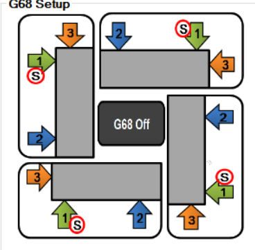
Position the probe tip at the approximate place shown by the S in the button, and press it. There are two methods, chosen with the G68 corner / edge options: Edge probes a single edge (two hits, using the Edge Length), Corner probes a corner (using the Corner Clearance to get around it; start closer to the corner than that distance).
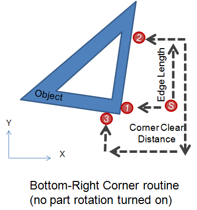
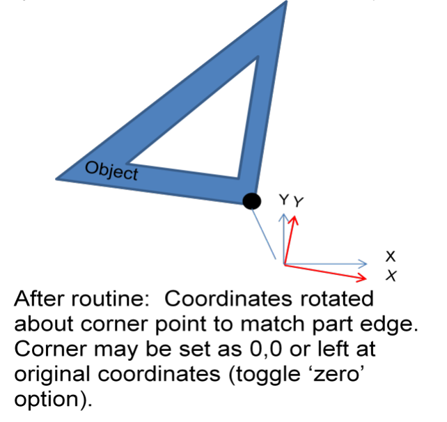
When the routine is done:
From now on every move is relative to the rotated system, until G68 is cancelled: click the LED button, or enter 0 in the angle box. The DROs go back to white when the rotation is cancelled. If G68 is already active when you start a routine, you are asked whether to clear it (G69) first. The G68 enable check box must be on before a G68 routine is run.
The Perimeter Probing page runs a routine that automatically follows the outside shape of an object and records the touched points, joined by lines, directly into a DXF file, or as X, Y, Z rows in a CSV file. It tries to always probe perpendicular to the surface and continually adjusts the probing angle. Probing square to the surface and using the tip table from the Probe Settings window lets the perimeter be reproduced accurately.
It works on both external and internal perimeters. It always works in the same direction: counter-clockwise around an external shape and clockwise around the inside of a pocket. Use the three sub-pages: XY Perimeter, XZ Perimeter (surface) and YZ Perimeter (surface) (section 11.4).
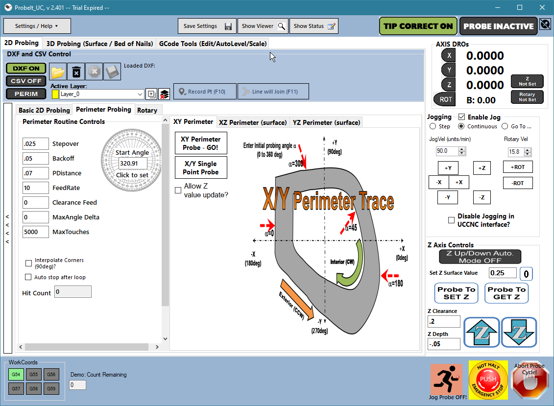
XY Perimeter → GO! starts the routine. Enter the settings, set the option LEDs, put the tip near the start of the perimeter of the object (at the proper depth), and press the button. It continues around until the maximum number of hits is reached, or the edge is lost in error. Use Abort at any time. You can reposition the probe and restart while recording to the same file; the data has a break in the curve where you restarted, which can be joined in the CAD program afterwards.
Single Point – Manual performs one probe event in the direction of the Initial Probing Angle. It is handy for collecting a few points around an object, or for adding points where the perimeter routine had difficulty. It records a point and a circle. The center of the circle is the part edge (where the tip touched), not the center of the tip: the tip radius offset is already included.
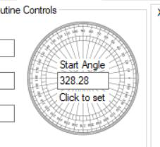
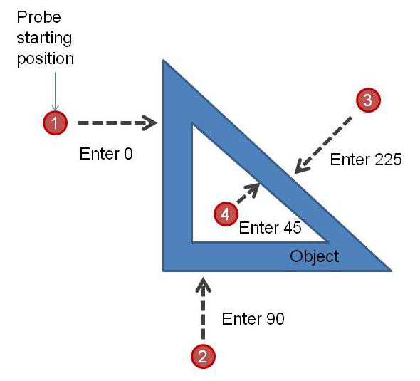
Initial Probing Angle. The angle (degrees) of the first probing vector from the current tip position, relative to the machine’s +X. Imagine polar coordinates with the origin at the tip, 0 degrees toward +X and 90 toward +Y. Click on the protractor to set it. Examples: probing +X when the probe is on the left of an outside perimeter: 0. Probing +Y from the bottom: 90. Probing −X and −Y toward a face at 45 degrees from the top right: 225. Probing +X, +Y toward a 45-degree face from the bottom left of an inner perimeter: 45.
Probing Feed. The probing feed. The perimeter routine probes at a single feed, one touch per hit (no back-off and slow re-touch). You can change it while the routine runs: use a fast feed for simple areas and slow down for complicated corners or to improve accuracy (less overtravel).
Clearance Feed. The feed for the clearance moves of the routine: backing off after a hit and returning to the last clear spot. The probing moves keep the Probing Feed, so the routine can probe slowly and still move quickly between touches. It can also be changed while the routine runs. Enter 0 (or leave it empty) to use the Probing Feed for these moves as well. It is separate from the Clearance Feed on the 2D probing pages. The XZ, YZ and rotary perimeter routines use the same two boxes.
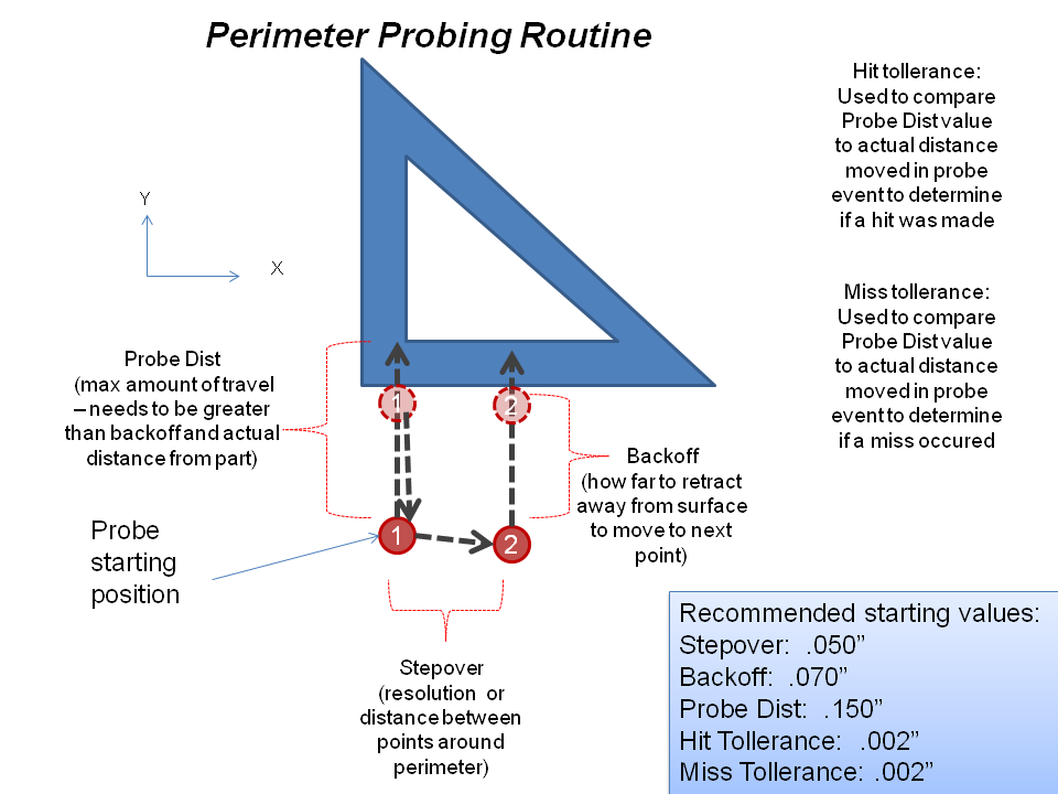
Stepover. The distance between probe points around the perimeter (actual points are only exactly this far apart along a straight line). A smaller stepover gives more samples and finer resolution. It cannot be changed while the routine is running: stop and restart it.
Backoff. How far the probe backs away from the surface to prepare for the next hit. It cannot be changed while the routine runs.
Probe Distance. How far the probe travels from the backoff point toward the surface. With the hit tolerance, it decides whether the surface was hit or missed. Always make it larger than the backoff, by about 1–3 probe-tip diameters. It cannot be changed while the routine runs.
Max Touches. The number of touches before the routine stops, so you can enter a large number and walk away. Estimate it as the approximate length of the perimeter divided by the stepover, plus about 20%. If it was not enough to get around the part, restart and keep recording to the same file, as long as you have not closed it; update the initial probe direction where you restart. In demo mode the routine stops at 1000 points. It cannot be changed while the routine runs.
Auto Start/Stop. With this on, probing stops by itself after completing a lap and returning to the start location.
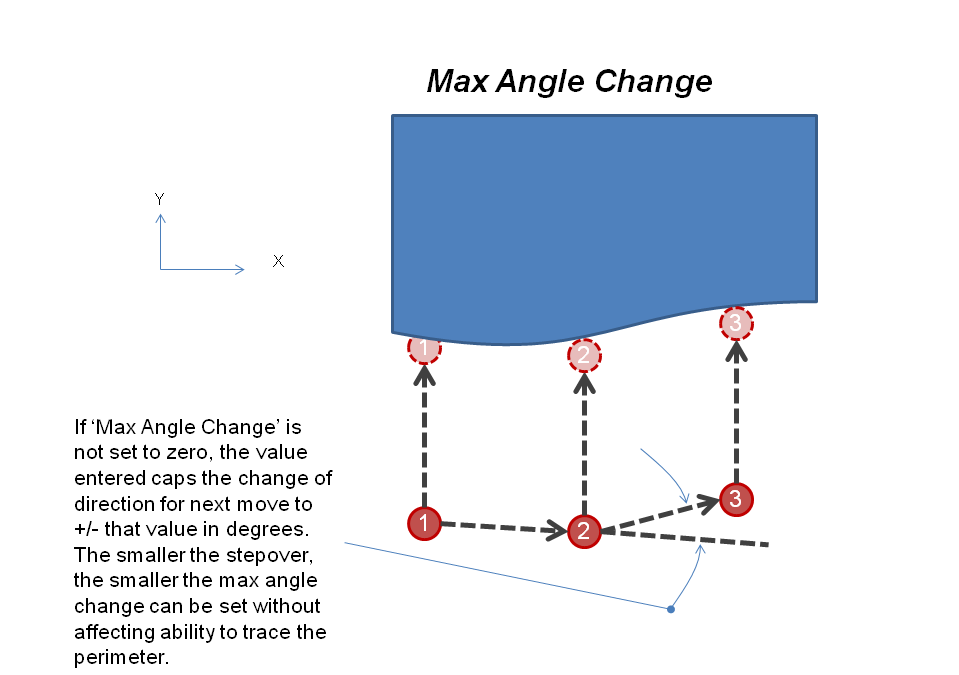
Max Angle Change. Limits how fast the routine may change direction: 0 disables it, 10 means the direction cannot change by more than 10 degrees (plus or minus) from one point to the next. Useful with a very small stepover, where small surface deviations cause large changes in the calculated angle and so errors in the data. It can be changed while the routine runs.
Error Message ON/OFF. With this on, a message interrupts the routine when:
These messages are useful while you learn how the routine works, and give you a pause to assess it. With the option off, the routine just keeps going. It can be turned on or off while the routine is running.
Interpolate Corner ON/OFF. With this on, an estimated corner point is inserted at an abrupt change of direction (for example when the probe misses and turns around a corner), assuming that the corner is square. The DXF/CSV then has a better representation of the corners, which you can correct in CAD. With it off, only real touch points are recorded, which may leave corners under-defined. It can be turned on or off while the routine runs.
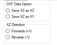
These routines probe along a surface in the X/Z or the Y/Z plane. The buttons and inputs are very much like the XY perimeter routine (see above). The differences:
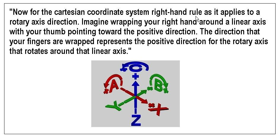
The Rotary page has routines that are handy for setting up parts on a 4th (rotary) axis. Enable and set up the rotary axis in the Rotary Axis group of the General Settings window: Enable Rotary Axis, Rotary Axis Letter, Rotary Axis is Parallel With. The routines assume:
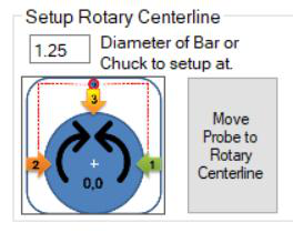
The routines rotate the rotary table (and move Z up and down if needed). X and Y stay as you positioned them (center the probe on the rotary centerline). They let you set the rotary angle to align with a feature on a shaft such as a keyway or ridge.
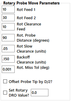
Rot Feed1, Rot Feed2 and Rot Clearance Feed are like Feed 1, Feed 2 and the clearance feed of the XY routines, but they are the tangential speed of the probe tip relative to the rotary at the current Z of the tip. Enter your native units per minute, not degrees per minute: the routines use the Z height of the tip (and Z = 0 at the centerline) to calculate the rotary feed. Feed 2 = 0 means no second slow hit. The clearance feed is used for transfer moves, such as moving sideways during the ridge routine.
Rot Probe Distance is like the XY probe distance, but in degrees of rotation: 90 lets the table turn up to 90 degrees to find an edge; if nothing is hit it stops and reports a miss. Rot Slow Clearance and Rot Backoff Clearance are in normal units (inch or mm); the rotation needed is calculated from the Z height.
Rot. Miss Tol (deg) is the miss tolerance of these rotary probe moves, in degrees. A rotary probe move that turns its whole angle, to within this tolerance, is a miss: nothing was touched. The default is 0.001. The rotary 3D grid has its own tolerance (section 15.2).
Z depth. The depth of the rotary probe moves is not set on this page. It is the Z Depth box in the Z Axis Controls on the main window, the same box the other routines use: the side probes go that far below the top of the part (the Z surface just probed). A note at the bottom of the rotary settings says so. Set it before running a rotary routine.
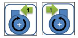
Rotary Side(s). Rotates the axis clockwise or counter-clockwise (depending on the button) and probes the side of a feature. Use it to make that feature vertical when the rotary DRO is set to a value you choose. With Offset Probe Tip by D/2 the tip moves off the centerline by its radius so that the wall can rotate fully vertical into the tip. Check Set Rotary DRO Value and enter a value to have the DRO set from the probing event.
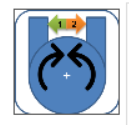
Rotary Slot. Rotates the axis clockwise and counter-clockwise inside a notch such as a keyway, then rotates back to the center and sets the axis DRO if chosen. Lower the probe into the groove by hand, and set a Rot. Probe Distance large enough for both sides to be touched.
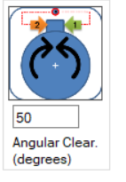
Rotary Ridge. Rotates the axis around a male key or tab and rotates back to the center, setting the DRO if chosen. Position the probe above the tab first. Set the Z Depth in the Z controls to how far down to go from the top. The routine probes down onto the top of the tab, moves to clear the tab by the Angular Clear. value, drops to the Z depth, and probes toward the outsides of the tab.
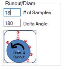
Rotary Roundness / Diameter. Sweeps the rotary clockwise or counter-clockwise over the Delta Angle: 180 for half a turn, 360 for a full turn. Over the sweep, Z probes down as many times as the # of Samples (18 samples over 180 degrees probes every 10 degrees). It then reports a measured diameter and roundness. The calculation assumes the axis centerline is Z = 0, so it is only as good as your centerline setup.
ProbeIt records probing data to a CSV file (comma-separated values, importable to Excel), to a DXF
file, or to both at once. Recorded files are saved in the output folder of the ProbeIt folder, for example
C:\ProbeItM3\output\. A third option, PERIM, records a simplified X/Y/Z perimeter file that the
3D probing page can use as a boundary.

Turn on DXF, CSV, or both. You are asked for a file name when you start; with both on, the name is used for both formats. Once the LED is on and a name is entered, you just probe: everything is recorded until you close the file. Record Perimeter captures the profile as data that the Surface / Grid Probing page can use as a containment perimeter.
output folder the first time. The folder is remembered between runs.The DXF format is standard and can be opened by any program that reads DXF. Geometry is drawn as points, lines, circles and so on. DXF files are suitable for VCarve and LightBurn: ProbeIt opens files exported from them and saves files they open. Layers and layer colors can be created, renamed, deleted and changed (see the viewer).
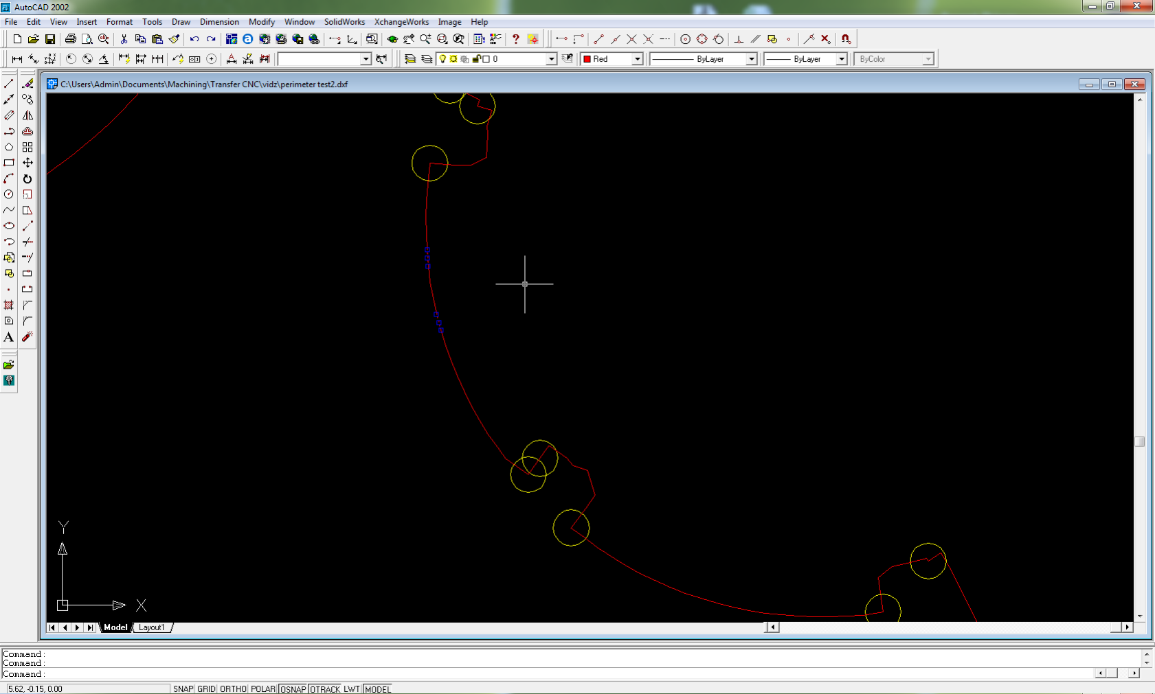
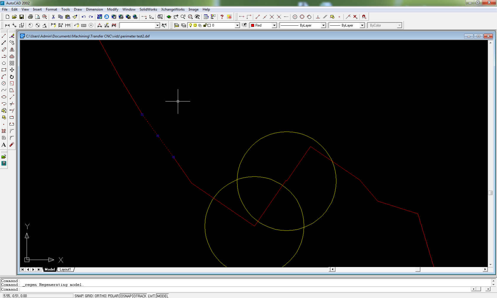
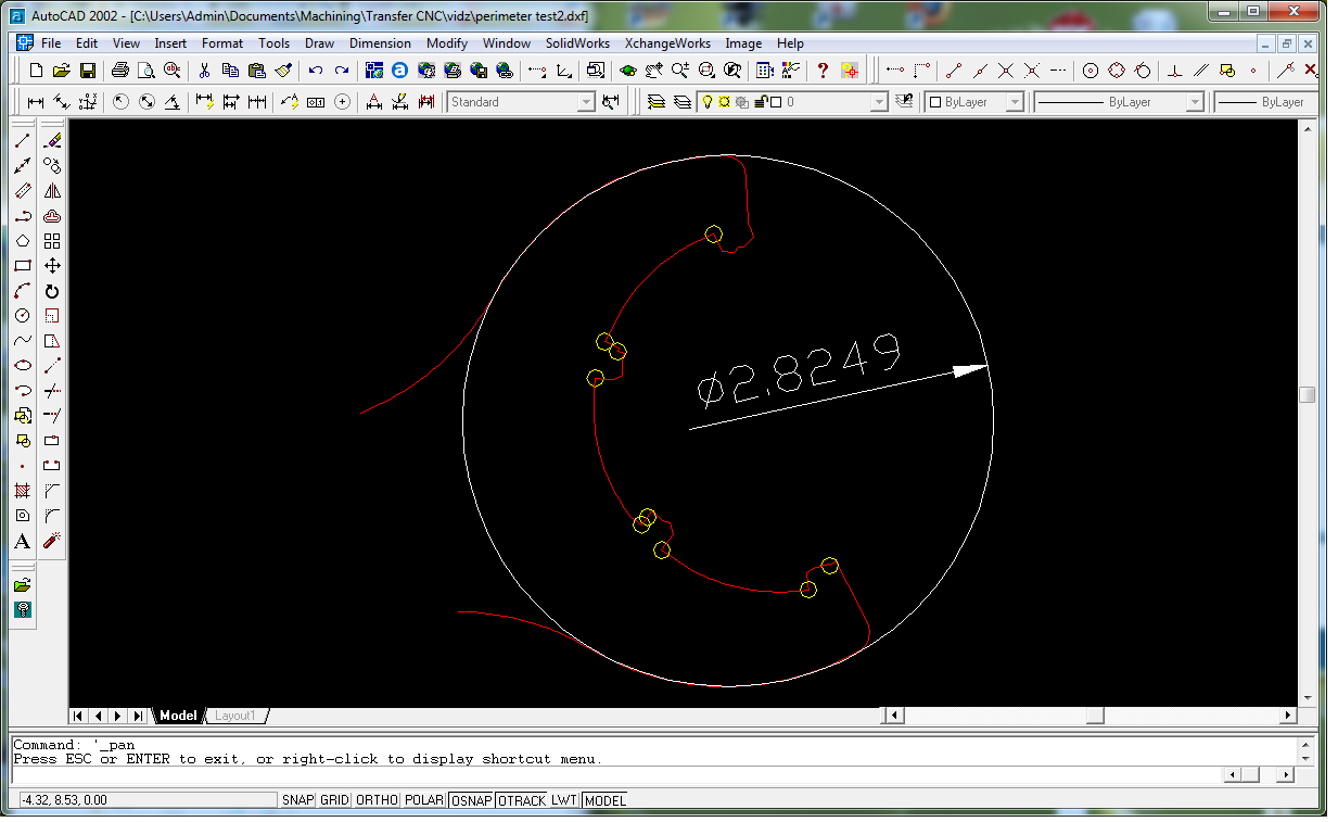
Perimeter probing creates a series of short line segments. A segment’s start and end points are the actual locations probed (as adjusted for the probe tip): the lines run along the true perimeter of the part and are not the center points of the probe ball. Occasionally, when a corner is found or missed during a direction change, the routine guesses and interpolates a corner point. These are drawn as small yellow circles whose center is the guessed location, and may need cleanup.
You can use the geometry to build better CAD geometry, join it into smoothed polylines, or import it into a CAM program to make cutting paths. You can measure by snapping circles and dimensions to the endpoints, or by curve fitting. Below, a recorded perimeter of an ER collet wrench: the red perimeter is many short segments, but the diameter is easily measured by building a 3-point circle that snaps to segments; the yellow circles mark guesses at abrupt direction changes.
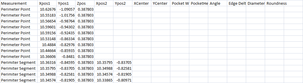
The CSV format is tabular and can be opened in Excel. It works well for simple CMM-style inspection: the diameters and locations
of a series of holes, for example. The program saves Filename.csv, where Filename is the name entered for the DXF. Each
row describes the probe event with the numbers; the example is a bore measurement, then perimeter data. In the perimeter data,
segments are short lines from a start point (Xpos1, Ypos1) to an end point (Xpos2, Ypos2).

The perimeter file (Filename_perim) is a very basic CSV with only X, Y, Z points and no header. It is meant to be
opened on the 3D probing page as a perimeter that bounds a point-cloud routine.
The GCode Tools tab has a full G-code editor and viewer. You can preview G-code files, edit them, and review the changes, and the toolbar has tools to:
Click a toolpath in the 3D view to select the matching line of G-code, and select a line to see it highlighted in the 3D view; selected moves show a direction-of-travel arrow, and hovering shows a preview highlight of the path under the mouse. Large G-code files load in the background without freezing the window.
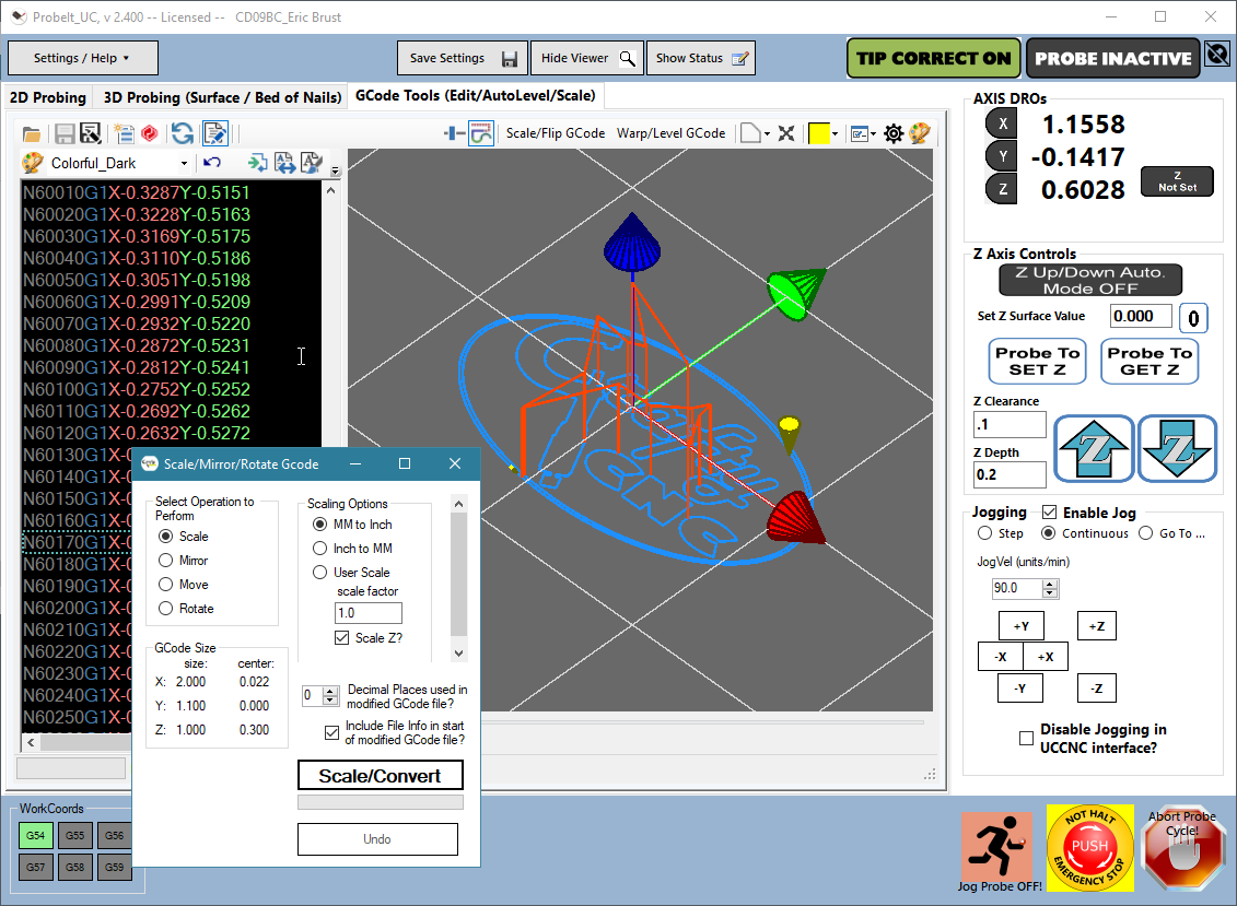
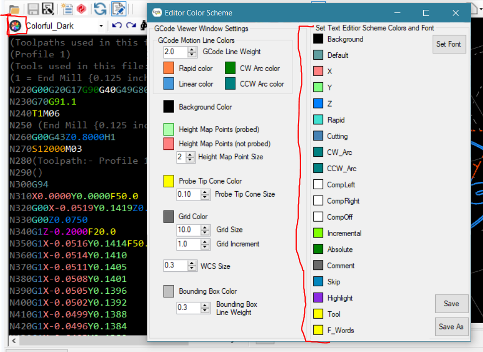
The text in the left panel can be edited by hand. Text colors can be customized in the color settings panel. The selected-line highlight color can be changed with the color picker.
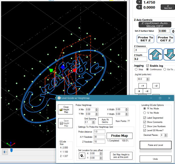
The Warp/Level GCode button opens a form that lets you autolevel (“wrap”) your G-code onto a surface that is not flat. First you need a height map that covers the area the G-code covers.
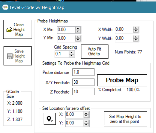
Use the Probe Heightmap settings to define a grid of points, and probe them for their Z values. Auto Fit Grid to GCode places a grid centered on the G-code with the spacing in Grid Spacing; you can adjust the Min X/Y, the widths and the spacing to cover the material better. Set the probe search distance and feed rates, and press Probe Map to collect the height map. You can also save a previously probed surface to an HMap file and re-open it later (use Save after probing, Open to reload).
Set Location for zero offset slides the height map up or down so that you can choose where zero is: move the machine to the location, press get location (or type X/Y), and press Set Map Height to zero at this point. No Z offset is applied at that point, and that is the place where you should then zero the bit before running the G-code. You can do this after loading or probing a height map, and save the map with or without the offset.
Once a G-code file is open and a height map is loaded (it must be 100% probed), you see the grid of points and the G-code together in the viewer.
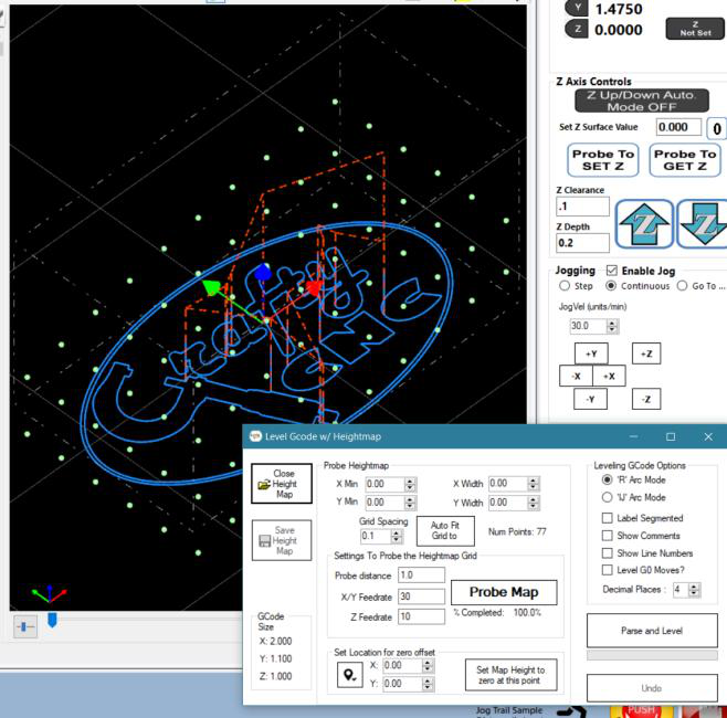
When the options are right, press Parse and Level. It processes the G-code and puts the new edited file in the editor and viewer. Undo reverts to the code before the last leveling, so you can change an option and run it again. If you are happy with the result, save it to a new file, or use Send to Mach3 to send it directly to Mach3. The original file is not changed until you save over it.
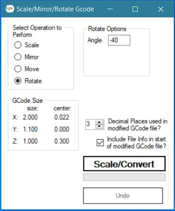
The Scale/Flip GCode button opens a form. Choose the operation:
You can choose the number of decimal places of the output G-code and whether to include a summary of the changes in the output. Press Scale/Convert to process; Undo reverts. Save the result or send it to Mach3: the original file is unchanged unless you save over it.
The 3D Probing (Surface / Bed of Nails) tab holds what used to be a separate plugin, ProbeCloud. It probes the surface of an item to make a CSV text file of X/Y/Z coordinates, the usual “point cloud”, with a bed-of-nails style routine. Unlike typical routines it does not just do a rectangular grid: it can probe only the points inside (or outside) a perimeter you define. You can even probe a perimeter to a file and open it as the boundary. Features that help with thousands and thousands of points:
The 3D Probing page is laid out in four numbered groups, in the order you use them: 1 Perimeter (optional), 2 Grid, 3 Probe Settings and Run and 4 Point Cloud (review or resume). The rough steps:
name.perim is saved. (You do not need to
jog back to the start: the last and first points are joined.)name.grid file; or load an existing one with Open Grid…. Once the grid file exists you are ready to probe.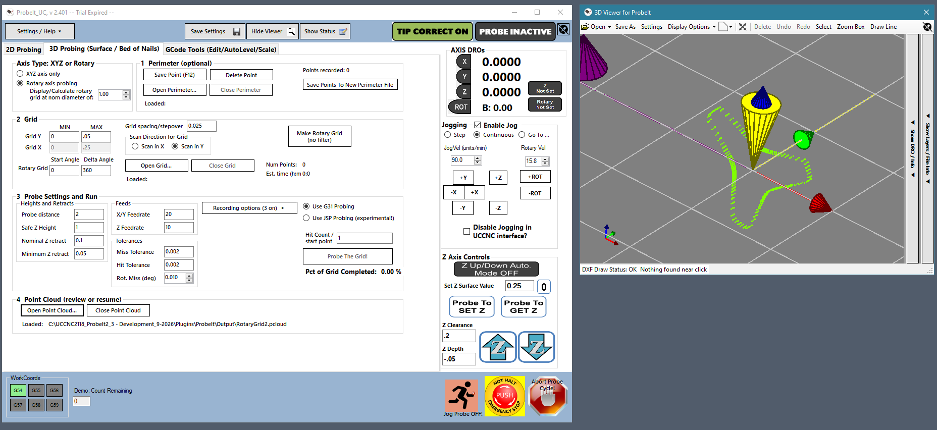
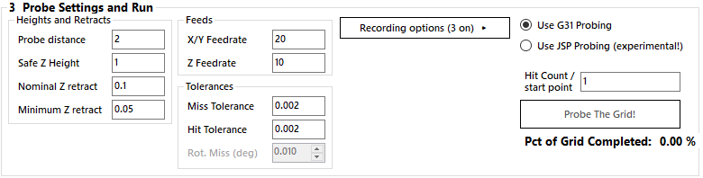
The settings of 3 Probe Settings and Run are in three boxes, plus the run controls:
| Setting | Meaning |
|---|---|
| Heights and Retracts | |
| Probe distance | The distance the routine attempts to probe in Z. The value is not important, as long as it is larger than the Z height of the part. |
| Safe Z Height | A plane above your part. The tip retracts to it only when necessary (for example if it hits the edge of the part during an X/Y move). |
| Nominal Z retract | How far the tip retracts, nominally, from the surface after a Z probe to move to the next point. The program keeps raising and lowering it according to the slope of the surface. |
| Minimum Z retract | The absolute minimum retract. The program varies the retract with the slope, but never below this. |
| Feeds | |
| X/Y Feedrate | The feed for the X/Y moves to the next point, all done as G31 probe moves at this feed. |
| Z Feedrate | The feed for the Z probe move (sampling the surface and recording). All Z moves are G31 probe moves at this feed. |
| Tolerances | |
| Miss Tolerance, Hit Tolerance | In your length units (the numbers shown are for inches; keep them small). Miss tolerance: the probe did not hit an object on a move where it was not supposed to (such as moving in X/Y to the next point). Hit tolerance: the probe hit an object on a move where it was supposed to (such as probing in Z to the surface). |
| Rot. Miss (deg) | The miss tolerance for the rotary grid, in degrees. It is greyed out unless Rotary axis probing is selected (section 15.2). |
| Run controls | |
| Hit Count / start point | The point number to start (or resume) from, from 1 up to the number of points in the loaded grid. It increases with each point recorded, so you can stop and restart. To start over, set it back to 1 before pressing Probe The Grid! |
| Recording options | A button that shows or hides four check boxes (its label shows how many are on): Log G-code Moves writes a log of every G-code command sent, for debugging (the log is written to the output folder as fname_gcode_log.txt); Empty Log on Every Start empties that log each time probing starts instead of adding to the previous run; Halt if a Z probe misses? stops the run when a Z probe finds nothing (leave it off if some points may be off the edge of the part); Record Position on Miss? records a position for a missed point, based on the starting height minus the probe distance. |
| Probe The Grid! | Starts the routine; the button turns into STOP. Press it to stop or pause, and again to restart. The routine runs until it is stopped, all the points in the grid file are collected, or an E-stop or feed hold occurs. Pct of Grid Completed beside it shows the progress. |
Your settings are saved with the main settings, using Save Settings.
Rotary grid probing creates a point cloud using the rotary axis. It is much like the XYZ routine, with these differences:
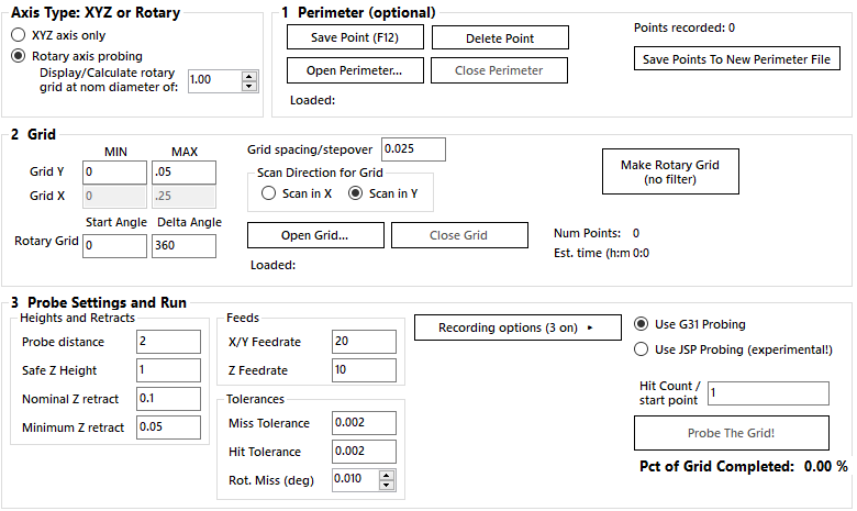
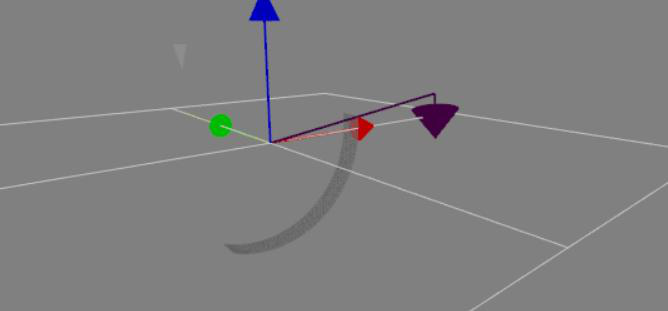
Rotary tolerance. The Rot. Miss (deg) box in the Tolerances group on the 3D Probing tab (next to Miss Tolerance and Hit Tolerance) is the angle version of the miss tolerance, in degrees, and is used only by the rotary grid. It decides whether a rotary move to the next point was stopped by a touch. The default is 0.01 (0.001 to 0.1 is allowed); a larger part radius turns the same angle into more travel at the surface. It is only enabled when the rotary grid is selected. If the tip touches during a rotary move, the routine lifts to the safe height, repeats the rotary move, and carries on; it stops with “probe stuck” only if the probe is still active after the repeat, or the axis is well short of its target.
If the rotary axis does not move at all (for example it is disabled or locked in Mach3, or the Rotary Axis Letter in the General Settings is not the axis that turns), the routine stops and says so, instead of reporting a stuck probe.
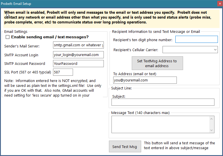
ProbeIt can send an email or text message on errors or when probing finishes successfully. Open Settings / Help → Email Setup….
| Setting | Meaning |
|---|---|
| Enable sending email/text msg | Turns sending on or off. |
| Sender’s mail server | The SMTP server to send through, such as smtp.gmail.com. |
| SMTP account login | The account, usually your email address. |
| SMTP account password | The password (or app password) for that account. |
| Port | The mail server port. 587 is typical. |
| Recipient’s ten-digit phone number, Recipient’s cellular carrier | ProbeIt only sends email, but you can text yourself through your carrier’s email gateway. Enter your number and pick the carrier from the list (for example @tmomail.net for T-Mobile), then press Set Text/Msg Address to fill in the To Address automatically. If your carrier is not listed, ask your provider for its gateway address. |
| To address | The address to send all messages to: a normal email address or a phone-number gateway address (8881234567@tmomail.net, for example). |
| Subject, Message | Used only by the test message. |
| Send Test Msg | Sends a test. You get a success message, or error information that points to something wrong with the server settings or login. |
During probing a message is sent if the target is missed and probing stops, the probe sticks on in the triggered state, an E-stop or feed hold happens, or the probing completes successfully.
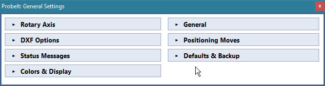
Open Settings / Help → General Settings…. The window has collapsible groups (click a group’s heading to open or close it; ProbeIt remembers which are open):
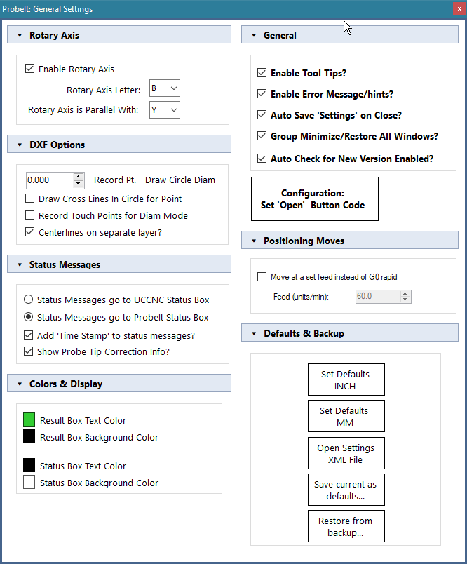
Use Save Settings to save all of the settings (every check box, number box and text box, and which groups are open) to the
ProbeIt.xml and ProbeItViewer.xml files in Settings\. If Auto Save on Close is on, they are
saved when ProbeIt closes. Settings are written safely (to a temporary file that is checked before it replaces the old one).
The starting values are built into the program, one set for inch and one for metric (the viewer’s grid and marker sizes follow your
choice). Set Defaults INCH and Set Defaults MM in the Probe Settings window load them again. Save current as defaults…
asks whether the current values are inch or metric and writes the current main-window and viewer settings (without your email
account and password) to Settings\Defaults\; those files then replace the built-in values for the Set Defaults buttons and for a new
install. Make sure the values really are in the units you choose.
Whenever a settings file is about to change, ProbeIt keeps a copy in Settings\Backups\ (the newest 10 of each file are kept).
Restore from backup… lists them and puts one back. If a settings file cannot be read when ProbeIt starts, you are offered the
newest backup; if you decline, the defaults are used and the damaged file is not overwritten by the close-time save. A line is added to
Settings\SettingsLoad.log for each settings load, and for every value that could not be applied: look there first if a setting does not
stick.
Press Abort. It halts any running routine, the basic XY routines and the perimeter routine included. If things are really going wrong, press the E-stop; you can always restart your probing after a reset.
If you are licensed (or still within the demo limits), you may stop and restart the perimeter routine as often as you need and keep recording to the same DXF or CSV file. You can mix XY routines with perimeter routines in one file; change stepover and backoff for more precision in some places and speed in others; and recover from an error where the routine lost the part or got hung up on a difficult spot. The recorded data has a broken line where the routine was restarted. It is easily fixed in CAD, as there are points at the line ends to join.
Yes. You can change the probing feed and the max angle change at any time. To change the stepover, backoff or other values, stop the routine (Esc), change them, and restart. It would be too risky to change the others on the fly, because they are used to determine the probe positions as it goes.
Look at the status line of Mach3: ProbeItM3 says there why it refused a command. It refuses when it was started read-only, when Mach3 is in E-stop, and (for probing) when Mach3 displays machine coordinates. Do not jog or send commands from Mach3 while a routine runs.
The routine turned the rotary axis and its position did not change. Check that the axis is enabled and not locked in Mach3, and that the Rotary Axis Letter in the General Settings is the axis that really turns.
Check the probe wiring and the probe input setup in Mach3. Do not run a routine until the LED turns on when you trigger the probe by hand and off when released.
The button and LED pictures are loaded from the images folder of the program folder. Re-run the installer to put them back. You can also replace
them with your own pictures of the same name.
Look at Settings\SettingsLoad.log (section 17.3), and use Restore from backup… if needed.
| Version | Notes |
|---|---|
| 2.401 |
First release of the Mach3 edition. The probing routines, recording, viewer and G-code tools of ProbeIt for UCCNC 2.401, running as a separate program next to Mach3 with a real Viewer: measuring
Viewer: editing
Viewer: other
Probing
|
The history of ProbeIt for UCCNC is in the UCCNC manual. The full list of changes for each version of ProbeItM3 is in README.txt, installed with the program.
| Item | Location (in the ProbeItM3 folder, C:\ProbeItM3 unless you chose another) |
|---|---|
| The program | ProbeItM3.exe and ProbeIt.Core.dll |
| Window-snapping helper and graphics library | MagnetWindows.dll, OpenTK.dll, OpenTK.GLControl.dll |
| Button and LED pictures | images\ |
| This manual | Manual\ProbeItM3-Manual.html |
| Settings (main window, viewer, G-code leveler and scaler, window positions, backups, log) | Settings\ |
| Saved defaults (override the built-in ones) | Settings\Defaults\ |
| G-code editor colors and machine files | Settings\EditorData\ |
| Recorded DXF / CSV / perimeter / grid files | output\ |
| Sample G-code, height maps and recordings | Gcode\ and Output\Samples\ |
| License agreement and install notes | PIT_EULA.rtf, README.txt |
| Trial and license | in the registry, HKCU\Software\CraftyCNC\ProbeItM3 (left alone by the uninstaller) |
ProbeItM3 is copyright CraftyCNC and E. Brust. ProbeIt and CraftyCNC are in no way affiliated with Newfangled Solutions.